Fluidized bed reactor CFD: which model, which drag law, how far to trust it
A revamp or scale-up decision waits on how bubbles, solids and tubes behave at plant scale, and the answer rests on a drag law, a mesh and a size distribution. Two-fluid, MP-PIC and CFD-DEM models, each used where valid and checked against your data, put bed, tubes and cyclone on one chain.
Fluidized bed CFD predicts how bubbles, solids circulation and heat transfer behave inside a reactor, so a distributor, tube bundle or cyclone loop can be compared before a pilot run or a shutdown window is spent. No single model answers every question: a two-fluid model carries the vessel, MP-PIC or CFD-DEM the grains where they matter, and each is only as good as its drag closure and validation. We set that chain up around your existing solver.
The pilot bed converted as predicted. The commercial vessel does not, its tube heat transfer is below the revamp case, and the bottom tube row is thinning faster than inspections expected. A distributor change, tube layout or cyclone modification is on the table, and each rests on one question: what do bubbles and solids do at this scale, with this powder?
What does fluidized bed CFD have to resolve inside a reactor?
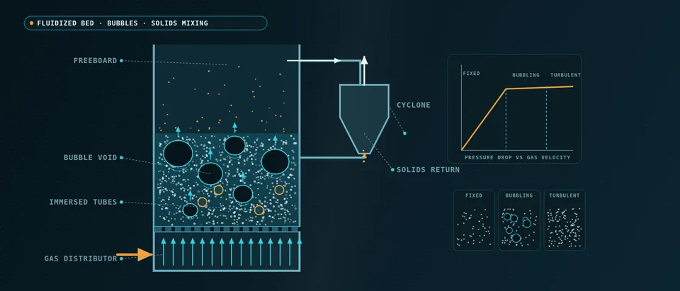
Below minimum fluidization the bed is packed and its pressure drop follows the Ergun relation, Δp/L = 150μ(1−ε)2U/(ε3d2) + 1.75ρg(1−ε)U2/(ε3d), with ε the void fraction, d the particle diameter and U the superficial velocity. At minimum fluidization that drop equals the bed weight per unit volume, (1−εmf)(ρp−ρg)g; beyond it the extra gas passes as bubbles. Geldart's 1973 groups say how a powder takes them: A expands first, B bubbles at once, C is cohesive, D is coarse.
Bubbles are what the reactor lives on. They bypass the dense emulsion, so conversion depends on gas exchange between bubble and emulsion; they coalesce as they rise, carry solids up in their wakes and erupt at the surface, throwing fines toward the cyclone. Your kinetics enter as species sources on top (see our detailed chemistry page). Hardy and colleagues (2023) note that the structures range from a few particle diameters to the vessel, up to 103–105 diameters, in beds of trillions of particles. Nothing follows them all, so each model chooses what to resolve and what to close.
- Distributor and jets. Gas enters through the holes of the distributor as jets, and the hole pattern sets the first bubbles. A distributor drawn as a uniform porous plate hides that; one drawn hole by hole costs cells, so the choice is made against the question: bubble size near the plate or behaviour of the bed above it.
- Bubbles that grow and coalesce. Bubbles are small near the plate and larger higher up because they merge as they rise. Gas that passes in bubbles bypasses the dense phase, so conversion depends on how quickly gas exchanges between bubble and emulsion. Bubble size and rise speed come from the closures and the grid, not from the equations alone.
- Solids circulation in the emulsion. Solids are carried up behind and between the bubbles and sink along the walls, a loop that mixes the bed. A model has to keep that loop and the wall layer right; a wall condition or a grid that damps it changes mixing and heat transfer together.
- Tubes and the wake impact. Tube bundles are struck by bubble wakes. Levy and Stallings found erosion caused by wake impact, highest when two bubbles coalesce directly beneath a tube, and a computed rate very sensitive to the height of the bottom tube row above the distributor. The same bubbles set the heat transfer to the tube.
- Freeboard and fines. Bubbles erupting at the surface throw grains upward, and the finest leave with the gas. The size distribution, not one mean diameter, decides what leaves the bed, so the size classes are an input to the model and to the cyclone loading.
- Cyclone and dipleg. The cyclone returns collected solids down the dipleg to the bed. Bed, cyclone inlet and return leg are one coupled loop: what the freeboard sends out sets the cyclone loading, and what comes back sets the inventory and size distribution of the bed. We keep that interface explicit in the model.
Two-fluid model, CFD-DEM or MP-PIC: which one does a fluidized bed need?
The two-fluid model treats gas and solids as interpenetrating continua, closed by kinetic theory of granular flow, a frictional stress near packing and a drag law; its cost follows the cell count, so it runs whole vessels. CFD-DEM follows every grain with contact forces; its cost follows the grain count and the contact time step. Di Renzo and colleagues (2021) quote CFD-DEM runs of 4.5 million particles in bubbling beds and 25 million on a GPU, against engineering systems of 108–1012 particles. MP-PIC sits between: parcels stand for many grains and the solids stress is modelled.
Neither is a quality ladder. On the NETL small-scale challenge bed, Lungu and colleagues (2021) ran both in one open-source code: the mean pressure drop ignored the drag correlation while fluctuating quantities did not, the two-fluid model was better for particle granular temperature, CFD-DEM for bubble granular temperature, and CFD-DEM took longer. On another small bed, Lu, Gopalan and Benyahia (2017) found MP-PIC predicted an unphysical particle overlap and wrong bed hydrodynamics, while hard-sphere collisions or parcels of a few particles kept accuracy at higher speed. One bed in one code is a reason to test a method on your powder, not a verdict.
- Two-fluid model. Gas and solids are interpenetrating continua in every cell, shaded here by solids fraction. The cost follows the cell count, so whole vessels are possible, but the solids stress and the drag between the phases are closures, and anything smaller than a cell is invisible to it.
- MP-PIC parcels. Parcels, each standing for many grains, are tracked on the same mesh, and the solids stress is modelled from the cell average rather than from contacts. It sits between the two-fluid model and CFD-DEM in cost. Its packing behaviour is the thing to test on a dense bed: one small-bed comparison found particle overlap and wrong bed hydrodynamics.
- CFD-DEM grains. Every grain is followed with contact forces, so mixing, segregation and wear mechanisms come from the grains themselves. The cost follows the grain count and the short contact time step, which limits CFD-DEM to small beds or to coarse-grained grains.
- One drag law closes all three. The gas-solid drag, the solids stress and the wall and inlet conditions feed every model. On a small test bed the mean pressure drop did not depend on the drag correlation while the fluctuating quantities did, so a drag law is checked against bubble statistics, not against the bed weight.
- A cluster inside one cell. Streamers and clusters smaller than a cell shift the real drag, and a coarse grid cancels them. Filtered models add a sub-grid drag correction for what the cells cannot see, physics-based or trained, and it has to be tested inside a coarse run, not only against fine-grid data.
- Coarse-graining. Bigger, fewer grains lower the CFD-DEM cost and bring pilot-scale beds within reach, but the grains then need scaled contact and drag laws and a coarser fluid mesh. How far the saving costs accuracy is, in a 2021 review, still not fully answered, so we state the grain-to-particle ratio with the result.
How much does the drag law change a fluidized bed simulation?
Drag is the closure every model leans on: Wen-Yu, Syamlal-O'Brien, Gidaspow (Wen-Yu when dilute, Ergun when dense), or structure-dependent forms such as EMMS that correct for unresolved clusters. Once a bed fluidizes its mean pressure drop is set by its weight, so matching it validates almost nothing about the drag law; bubble frequency and solids-velocity fluctuations do.
Storlie and colleagues (2014) show a disciplined calibration. For a 48 × 60 × 34 cm bubbling bed with twenty-five 2.54 cm tubes, a two-dimensional model carried six uncertain inputs, the drag model a categorical one, over 90 designed runs, scored on bubble frequency and bubble phase fraction from a probe on one tube. Wen-Yu was chosen in nearly every posterior sample, and some discrepancy from the measurements remained. That describes one bed and powder; for yours we record the drag law as a calibrated choice, never a default.
The mesh is the second hidden closure. Hardy and colleagues say accurate two-fluid runs often need cells a few particle diameters wide, which vessels of 103–105 diameters cannot afford, so plant-scale runs use filtered models with a sub-grid drag correction. We run the mesh study on a bench-sized slice, then state which closure carries the plant-scale run.
How do immersed tubes, erosion and heat transfer change the model?
Levy and Stallings (Lehigh University and EPRI, 1991) report cold-model data showing erosion caused by bubble wakes striking the tubes, worst when two bubbles coalesce beneath one, and a simulation whose erosion rate is very sensitive to the height of the bottom tube row above the distributor. The same bubbles set heat transfer: the probe above also recorded contacting time. We hand tube temperatures and impact exposure to thermal and durability analysis, and treat an erosion prediction as a ranking of layouts until your inspection data calibrate it.
The loop matters as much as the bed. Fines leaving the freeboard load the cyclone and the dipleg return sets the bed's inventory and size distribution, so they are one coupled problem. A powder is a distribution, not a diameter, and carry-over is what a mean diameter hides, so we model the size classes your sieve data give.
Why does a small test cell mislead the scale-up of a fluidized bed?
Bubbles coalesce as they rise until they approach the vessel width, and then the bed slugs, so a bench cell partly measures its own walls. Vessel-to-particle size ratio, aspect ratio and gas velocity relative to minimum fluidization cannot all match the plant in a small cell, and plant gas at temperature and pressure has other density and viscosity than rig air, which by the Ergun relation moves minimum fluidization.
So we calibrate and verify closures on fine-mesh or resolved-grain runs of a bench-sized bed, run the vessel with the model its size allows, and record what the plant-scale run extrapolates. Verification is mesh and time-step convergence over a window long enough to converge; the calibration above ran 60 s and discarded the first 30 s as start-up. Validation uses your pressure signals, bed expansion and probe records, tolerances set beforehand.
Which fluidized bed question needs which model?
| Question | Model | What it reports | Limit to state |
|---|---|---|---|
| Bed expansion, bubble statistics, pressure fluctuations | Two-fluid model, calibrated drag | Time-averaged and fluctuating fields | Closures set the bubbles |
| Plant-scale bed with cyclone or wide section | Filtered two-fluid or parcel method | Circulation, inventory, carry-over | Sub-grid drag stands in for clusters |
| Mixing, segregation, collisions, wear | CFD-DEM, coarse-grained if large | Grain paths, contact forces | Grain count sets the cost |
| Dense mid-size bed needing grains | MP-PIC | Parcel fields, circulation | Test packing and overlap |
| Tube erosion and heat transfer | Two-fluid or CFD-DEM near tubes, wear model | Impact exposure by location, then FEA | Ranks layouts, not wall loss |
| Many distributor and tube variants | Surrogate on designed runs | Time-averaged outputs | Valid in sampled range only |
Where does AI help fluidized bed CFD, and where does it not?
- Closures for coarse meshes. Hardy and colleagues train neural networks on fine-mesh two-fluid runs in periodic domains, with filter size, filtered solids fraction, slip velocity and pressure gradient as inputs. The inputs that worked for dense beds worked for dilute flow, and the next step they name is running the closures inside coarse simulations. Earlier fits assumed no inter-particle forces, which change the correction, so a cohesive powder lies outside what is shown. We use such a closure only after that test.
- Calibration with an emulator. The Storlie approach, an emulator of designed runs with a discrepancy term and the drag model as a categorical input, returns a posterior range for your bed, not one tuned constant.
- Parametric reduced models. A 2023 SISSA study reduced a lab-scale CFD-DEM bed over Stokes numbers from 200 to 300, with mean errors near 12% at best on held-out values of gas volume fraction and the particle phase left for later. Bubbling is chaotic, so we aim surrogates at time-averaged outputs such as bed expansion and bubble frequency.
AI does not repair a wrong drag law, extrapolate to another powder or replace pilot data. See surrogate models for CFD and FEA, validating surrogates and our surrogate modelling, uncertainty quantification and hybrid physics-AI pages.
A fluidized-bed simulation is not a performance guarantee
From one bed study to a fluidized bed workflow you keep
The return comes when your engineers can run the next powder, distributor or vessel through the same chain.
- Physics model. CFD and FEA set up once, as templates: geometry clean-up, mesh, solver settings and post-processing that every later run reuses.
- Validation. Mesh and time-step studies, and comparison with tests or full-scale data, so the model's uncertainty is known before it is trusted.
- Automated runs. Scripted runs over the parameters and operating conditions that matter, on your hardware or in the cloud.
- AI surrogate. A machine-learning model trained on those runs answers in seconds and says how sure it is; low-confidence questions go back to the solver.
- Decision tool. Optimisation, trade-off charts or operating guidance, in a form your engineers and operators use every day.
- Field data. Test, trial and monitoring data flow back to recalibrate the model, so it improves with every project instead of being rebuilt.
- A parametric bed model in your existing solver (Ansys Fluent, Siemens STAR-CCM+, OpenFOAM): distributor, internals and cyclone inlet as parameters, choices recorded.
- A powder record of size classes, density and measured minimum fluidization velocity.
- A closure and mesh study on a bench-sized slice, with the drag comparison and its discrepancy on file.
- A validation record against your pilot or plant data, tolerances set before the run.
- A load-transfer post-processor handing tube temperatures and impact exposure to structural analysis.
- A surrogate with a stated range over distributor, tube layout and gas velocity, gated to the full model outside it.
- Handover and training so your team runs and extends it: see our training and software development services.
Questions engineers ask about fluidized bed CFD
Is a two-fluid model or CFD-DEM better for a fluidized bed?
Which drag law should I use?
Can CFD predict bubble size and bed expansion?
Can a bench-scale CFD model be scaled up?
Can CFD predict tube erosion?
If a revamp or scale-up decision is waiting on a fluidized-bed answer, send us the powder's size distribution, density and minimum fluidization velocity, the vessel drawing with distributor, internals and cyclone, the operating gas properties and any pilot or plant measurements. We reply with the model chain we would set up for each question, its validation record and what a surrogate could cover. Start with a conversation, or read our multiphase simulation page and chemical processing overview.