Rubber finite element analysis for tyres, hoses and mounts, from tests to fatigue
The compound passed its tensile test, and the part still stiffens wrongly, runs hot or cracks at a ply edge. Multi-mode calibration, cord-layer models, rolling heat and tearing-energy fatigue show which input is responsible.
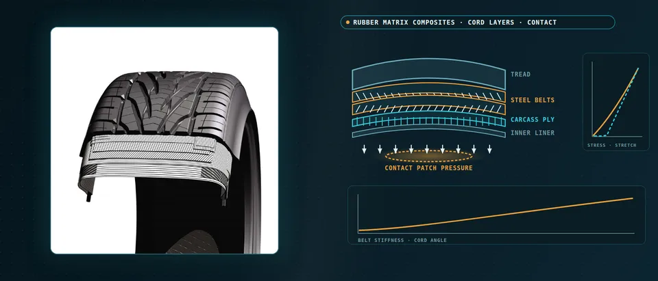
Rubber finite element analysis predicts how a tyre, hose, seal or mount deforms, heats and cracks once the compound’s hyperelasticity, softening and hysteresis, and the cord layers inside it, are modelled as they behave. We build it as a repeatable workflow around your solver, from multi-mode calibration to a validation record and a surrogate of stated range, so more of a compound or belt question is settled before the next mould, build or rig run.
The compound passed its tensile test, and the part still stiffens wrongly in shear, runs hot in the crown or cracks at a ply edge. Each answer has cost a mould, a build and a rig run, and the compound release and the launch date wait on the next. Usually one input is behind it: a model fitted on a single test mode, a cord layer smeared into a sheet, or a heat source never fed back into the stiffness.
Why is rubber finite element analysis harder than steel or plastic?
Three behaviours share every element. Large-strain elasticity first: rubber stays elastic at several hundred per cent extension and is nearly incompressible, so the strain energy splits into a volume-preserving part and a volume penalty, W = Σ(μi/αi)(λ1αi + λ2αi + λ3αi − 3) + (K/2)(J − 1)2 for an Ogden form, with λ the volume-preserving stretches. Then softening: a filled rubber’s first loading is stiffer than every later cycle, the Mullins effect, and Diani and colleagues (2009) find no general agreement on its physical source or its modelling. Last, hysteresis: each cycle loses energy as heat, depending on frequency and temperature. Tabaddor’s NASA conference paper (1989) adds that incompressibility grows less accurate as carbon black rises, so the bulk response is measured, not assumed.
How do you calibrate a hyperelastic model from rubber tests?
A uniaxial curve cannot fix a three-dimensional model: a part sees tension, shear and equibiaxial stretch at once. We calibrate on uniaxial, planar and equibiaxial tests of the same compound, cured and preconditioned as the part is, fitted together. Linka and Kuhl (2022) trained a constitutive neural network on classic rubber benchmark data in those modes: uniaxial data alone gave a non-unique fit, which they attribute to data that are not rich enough, and all three gave one model and one parameter set. For Mullins softening we decide what the part needs, the virgin or the stabilised response, and record the conditioning. A mount also needs modulus and loss against amplitude, frequency and temperature; a hyperelastic fit has no loss.
The element matters as much as the law. Displacement-only elements lock on near-incompressible rubber, stiffness too high and pressure noisy, so we use mixed displacement-pressure formulations and prove them on a confined-compression check. Tabaddor notes that Lagrange multipliers add unknowns and can ill-condition the stiffness matrix, and that large penalty numbers bring their own trouble, so the formulation is a recorded decision.
How do you model cord layers and belts in rubber?
A cord is a structure, twisted from yarns of filaments, and Tabaddor lists what follows: its effective properties change once embedded in rubber, differ in tension and compression, and are often nonlinear and viscoelastic. The contrast is the difficulty, a cord-to-rubber stiffness ratio that can exceed 30,000 in some composites, so homogenisation bounds sit far apart and we take ply properties from tests. A belt is two plies at ±θ. Under a pull the cords rotate toward the load, the angle between the plies changes, and the response turns nonlinear in a way a fixed-fibre model cannot show; the rubber between the plies carries that shear. A hose has its own neutral angle: pressure loads the hoop direction twice as hard as the axis, so at θ = arctan √2, about 54.7° from the axis, the cord net alone balances it. Scale choice is in our composite modelling article.
- Cord angle sets the load directions. Cords are stiff and rubber is soft: Tabaddor (NASA conference paper, 1989) reports a cord-to-rubber stiffness ratio that can exceed 30,000 in some composites. Load runs along the two cord directions, at plus and minus θ, so circumferential, lateral and shear stiffness all follow the angle.
- Under a pull the lattice scissors. Faint lines are the cords at rest, solid lines the same belt after a pull along the circumference: the cords rotate toward the load. The angle between the cords of adjacent plies changes, which makes the response nonlinear, so a fixed fibre direction is the wrong model for a belt.
- Rubber between the plies takes the shear. Opposed ply motion, the two arrows, shears the thin interply rubber. It is nearly incompressible and confined between stiff cords, so it sets the scissor stiffness and is where volumetric locking shows first. Tabaddor notes that filled rubber is less incompressible than unfilled rubber, so its bulk response is a parameter to measure.
- Ply edges are stiffness jumps. Where a ply ends, stiffness changes abruptly. Tabaddor notes that displacement-based finite element stresses turn very erratic at such changes, the cord-rubber interface among them, so edge strain is reported only after the mesh has converged.
- Soft scissor, then stiff cords. A qualitative curve: belt force rises slowly while the lattice scissors against interply shear, then steeply once the cords have aligned with the pull and carry it themselves. Where the load of interest sits on that curve decides which parameter the answer depends on.
- Three ways to build the belt. Tabaddor's element table: membrane layers need two-dimensional properties with the interplies modelled separately; one solid element per ply and per interply needs no update as the cord angle changes; lumped plies and shell sections use fewer elements but must update properties as it changes. Homogenised elements should not be smaller than the cords.
Modelling follows the question. A rebar or membrane layer is economical for global stiffness; solid plies with solid interply rubber resolve the shear and the ply edge. Tabaddor’s element table adds that lumped plies and shell sections must update properties as the cord angle changes, and that homogenised elements should not be smaller than the cords. Stresses turn erratic where stiffness jumps, so edge strain is reported only on a converged mesh.
How are tyre contact, heat build-up and rolling resistance simulated?
The footprint pressure is a result of belt, inflation, load and friction, so it is solved with the cord layers in the model. Steady-state rolling follows the material through the patch and is economical at constant speed; transient or explicit rolling covers events, and our tyre hydroplaning article picks up the water. Heat follows from the cycle: each element sees one strain cycle per revolution and loses πE″ε02 per unit volume for a sinusoidal strain of amplitude ε0. Clark and Dodge (NASA contractor report, 1982) turned that loss into a heat source, solved the diffusion equation with wheel and runway boundaries and compared it with buried thermocouples in aircraft tyres. Temperature then moves moduli and loss: a loop, not a post-process.
Rolling resistance holds a part a structural model alone misses. Hoever and Kropp (2015) split simulated loss into tyre structure and small-scale tread deformation on road texture: the structure part varied little with the surface, while the tread part was negligible on a smooth one and nearly half the total on the roughest.
How do you predict crack growth and fatigue life in rubber?
Fatigue is governed by tearing energy, T = −∂W/∂A at fixed displacement, the energy released per unit of new crack area. Below a threshold T0 cracks do not grow; Rong and colleagues (2021) measured it by cutting and by fatigue crack growth, and the two values differ a little, so we carry a range. In an intermediate band da/dN = rc(T/Tc)F, and Luo and colleagues (2019) found for one carbon-black-filled natural rubber that Tc fell exponentially from −40 to 70 °C, which ties fatigue to the heat loop. The model supplies T for cracks seeded where strain energy peaks. Life also depends on a cycle’s minimum as well as maximum strain, as the early natural-rubber data Tabaddor reproduces show, so load cases carry the strain ratio. See our elastomer fatigue page.
- One strain cycle per revolution. A rubber element enters the contact patch, deforms and leaves once per turn, so its strain history is a cycle at the rolling frequency. The orbiting dot marks one element. Steady-state or transient rolling decides how that cycle is obtained.
- Softening, then a loop. First loading follows the dashed virgin curve; after Mullins softening the cycle settles below it, and Diani and colleagues (2009) find no general agreement on its source or modelling. The shaded loop is the energy lost per cycle: π E″ ε0² per unit volume in a uniaxial cycle of strain amplitude ε0 (Clark and Dodge, NASA contractor report, 1982).
- Loss becomes heat, heat changes the rubber. The heat source q is the lost energy density times the rolling frequency. Clark and Dodge solved the diffusion equation for an aircraft tyre with wheel and runway boundaries and compared it with buried thermocouples. Moduli and loss depend on temperature, so the last box, stiffness E′ and tear resistance Tc, feeds back to the first.
- Heat gathers where strain energy is high. The warm patches mark where the lost energy density is largest; their place depends on design, load, pressure and speed. Rubber conducts heat poorly, and it leaves through the tread, sidewall and liner to air, rim and road. Those boundary conditions are inputs we calibrate.
- Crack growth: threshold, power law, ceiling. In tearing energy T, the energy released per unit of new crack area at fixed displacement, cracks do not grow below T0 (Rong and colleagues, 2021) and grow as a power law in an intermediate band. Growth turns unstable at the critical Tc, which fell with temperature in the filled natural rubber Luo and colleagues (2019) tested: the dashed hot curve.
- Rolling loss has two parts. Hoever and Kropp (2015) simulate the losses of the tyre structure and of small-scale tread deformation on road texture. The structure part varied little with the surface; the tread part was negligible on a smooth one and nearly half the total on the roughest. A model of the structure alone misses that share.
Which rubber question needs which model?
| Question | Model | Reports | Limit to state |
|---|---|---|---|
| Does stiffness hold in every load direction? | Multi-mode hyperelastic fit, mixed elements | Stiffness, local strain | Modes tested; strain range |
| How far does the first stroke differ from service? | Softening model, conditioned specimens | Virgin and stabilised response | Origin unsettled |
| Where does the belt strain at its edge? | Rebar layer, or solid plies with interply rubber | Edge strain energy, interply shear | Cord properties; edge mesh |
| What is the footprint pressure? | Inflated, loaded model with friction contact | Pressure and area maps | Friction law |
| Where does the crown heat up? | Rolling model, hysteresis, thermal solve | Temperature field, loss | Loss data against frequency, temperature |
| Where does a crack start, and how fast does it grow? | Strain-energy peaks, tearing-energy growth law | Critical sites, growth per cycle | Threshold range; temperature |
| Sweeps over belt angle, compound, geometry | Surrogate on designed runs | Stiffness, pressure, temperature maps | Sampled range; gate to full model |
A calibrated rubber model is not an approved part
Where does AI help rubber component design, and where does it not?
- Model discovery. The network of Linka and Kuhl selects among classical rubber models and fits their parameters from multi-mode data, built to respect objectivity, thermodynamics and polyconvexity. Their cases are perfectly incompressible and isotropic; history-dependent softening is a stated extension. We use it to screen model forms and show how far the data decide.
- Surrogates over belt angle, compound and geometry. Trained on designed full-model runs, they return stiffness, footprint pressure, edge strain energy and crown temperature in a stated range, gated to the full model.
- Inverse calibration. Automated fitting of loss and friction parameters to your rig data, within physical bounds, with the residual shown.
- Uncertainty. Compound scatter, threshold range, friction and ambient temperature become input distributions; the answer is a range with ranked contributors.
It does not supply a missing test mode, a softening law the physics has not settled, or a cure state the specimens never had, and networks fail to extrapolate beyond their training regime, as Linka and Kuhl state. Ours state their range and send other cases to the full model. See our surrogate modelling, hybrid physics-AI and uncertainty quantification pages and our articles on surrogate models and validating them.
From one rubber study to a workflow your team keeps
The return comes when your engineers run the next compound, belt layout or mount through the same chain.
- Physics model. CFD and FEA set up once, as templates: geometry clean-up, mesh, solver settings and post-processing that every later run reuses.
- Validation. Mesh and time-step studies, and comparison with tests or full-scale data, so the model's uncertainty is known before it is trusted.
- Automated runs. Scripted runs over the parameters and operating conditions that matter, on your hardware or in the cloud.
- AI surrogate. A machine-learning model trained on those runs answers in seconds and says how sure it is; low-confidence questions go back to the solver.
- Decision tool. Optimisation, trade-off charts or operating guidance, in a form your engineers and operators use every day.
- Field data. Test, trial and monitoring data flow back to recalibrate the model, so it improves with every project instead of being rebuilt.
- A calibration pipeline: test files in; parameters, a fit plot for every mode and the strain range of the fit out, versioned with compound, cure and conditioning.
- A parametric part template in your solver (we work with Abaqus, Ansys, LS-DYNA, RADIOSS and COMSOL): section, compound, cord layers, elements and rolling set-up in one file.
- A coupled chain from strain energy to heat, temperature and crack growth, with loss and tearing data in a library, each entry with source and range.
- A validation record against the footprint, stiffness curves, temperatures and rig results you hold, tolerances set before the run.
- A surrogate with a stated range and a gate to the full model.
- Handover and training, so your team runs and extends it: our training and software development services.
How credible is a rubber simulation result?
Verification is convergence: strain at ply edges and in thin rubber layers, element formulation, contact discretisation, time step. Validation uses what you hold or can generate: stiffness in more than one direction, footprint pressure, surface temperatures, one condition kept back. Uncertainty is sampled, as Tabaddor’s call for sensitivity analysis asks: compound batch, cure, loss data, threshold, friction. The answer is a range with ranked contributors.
Questions engineers ask about rubber finite element analysis
Which hyperelastic model should I use for rubber?
What is volumetric locking and how do I avoid it?
Do I need to model every cord?
Can simulation predict tyre rolling resistance?
Does simulation replace component or tyre testing?
If a compound release, a belt layout or a mount durability result is waiting on this, send us the compound’s test curves in every mode you hold, the section drawing with ply and cord data, the load cases and the failure you see, and any rig or temperature data. We reply with the model chain we would set up, the validation we would run and what a surrogate could cover. Start with a conversation, or see our rubber-matrix composite page.