Chemical reactor CFD for mixing-limited selectivity and exothermic hot spots
The pilot reactor makes more by-product than the flask did, and the peak temperature is not where the one-dimensional model put it. Reactor CFD with kinetics, a micromixing closure and a resolved wall shows whether mixing or chemistry limits selectivity and where heat removal falls short.
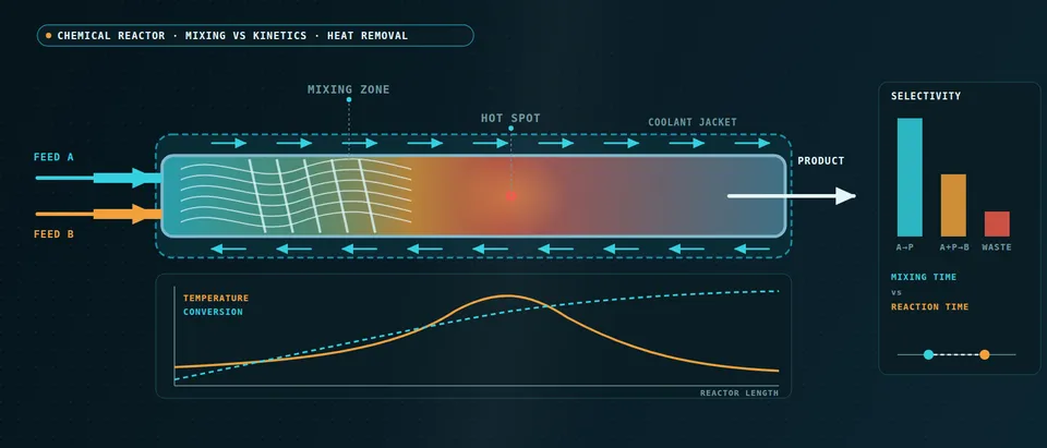
Chemical reactor CFD couples flow, species transport and the energy balance, so you can see where mixing rather than kinetics limits selectivity and where heat release outruns heat removal. It answers what a laboratory kinetic fit cannot: what the same chemistry does when the feed point, agitation or geometry changes at scale. We set it up around your existing solver and kinetic data, with a validation record and a surrogate of stated range.
The scale-up run is booked. In the flask the selectivity was acceptable; in the pilot reactor the by-product is higher and the peak temperature is not where the one-dimensional model put it. Nobody can say whether to blame the kinetics, the feed pipe or the jacket, and the feed location, addition time or coolant set-point waits on it. Akiti and colleagues (2005) note that the glass reactors used to fit drug-synthesis kinetics are usually assumed perfectly mixed. In their semi-batch experiments impeller speed and type changed the outcome significantly, the CFD dissipation rate at the feed point correlated with the measured segregation index, and mixing effectiveness fell appreciably between two laboratory vessel sizes.
When does mixing, not chemistry, set reactor selectivity?
Take two fast steps: A + B → R, the product you want, and R + B → S, the by-product. Where fresh B meets A, R forms; where B stays segregated beside R-rich liquid, S forms. What decides is a Damköhler number for mixing, Da = τmix/τrxn, with τrxn = 1/(kc) for a second-order step. When Da is small, chemistry decides and a kinetic fit transfers; when it is large, the fit alone cannot predict selectivity. Manzano Martínez and colleagues (2017) state it for competing reactions: micromixing time should be below reaction time, and in extremely exothermic reactions poor micromixing can also cause local hot spots.
Micromixing runs from the Kolmogorov scale down to the Batchelor scale, ηB = η/√Sc, and in liquids Sc is of order 103. Schikarski and colleagues calculate that resolving the Batchelor scale in a 1 mm T-mixer at Re = 4000 (Sc = 600) would take over 6 × 10¹² grid points, against almost 200 million for the flow itself. No plant mesh gets there, so a closure carries the last scales. In the engulfment model the micromixing time scales with (ν/ε)1/2, so the local dissipation rate at the feed point is the number to get right.
- Feed at the surface. A pipe that discharges into the slow core of a circulation loop leaves the plume to be dispersed by the large-scale flow alone. The reagent stays concentrated beside liquid already rich in the wanted product, so the second step runs and the by-product forms at the rim. The pulsing dots mark the wanted product made at the edge and the by-product made where the reagent is still in excess.
- Feed at the impeller discharge. The same feed placed where the local dissipation rate is highest is torn into thin sheets and carried round the loops. Akiti and colleagues found that the CFD-predicted dissipation rate at the feed point correlated with the measured segregation index, so the mesh has to resolve that region and the feed pipe itself.
- Lamellae from engulfment to diffusion. Large eddies engulf the plume, shear stretches the folds into sheets and molecular diffusion finishes the job at the Batchelor scale. Reaction happens at the interfaces, so by-product forms while the sheets are still thick. In liquids the Batchelor scale is smaller than the Kolmogorov scale by the square root of the Schmidt number, and no plant-scale mesh resolves it, so a closure carries it.
- Competing steps. A with B gives the wanted R; R with B gives the by-product S. Both are fast, so which one wins depends on whether fresh B meets A or meets R. That is a statement about mixing time against reaction time, so a kinetic fit alone cannot say which wins in your vessel.
- Selectivity against mixing time over reaction time. With mixing much faster than reaction the chemistry decides and selectivity sits on the left plateau. As the ratio grows it falls toward a plateau set by mixing. Scale-up tends to move the operating point right; a feed at the impeller, a slower feed or more power moves it left. The travelling dot is the sweep a surrogate would cover.
- What the model has to carry. Because the last scales cannot be meshed, the model transports the scalar variance and its dissipation, or a composition distribution, alongside the flow, and it needs the dissipation rate at the feed point and both rate laws. The closure is calibrated on a test reaction in a resolved region, then used in the full vessel.
How does chemical reactor CFD handle turbulence-chemistry interaction, and where does it fail?
The rate is nonlinear in concentration and temperature, so the mean rate is not the rate at the mean: ⟨kcAcB⟩ ≠ k⟨cA⟩⟨cB⟩. The gap is the unmixedness that every closure models. The cell-mean rate treats each cell as perfectly micromixed: right only when chemistry is slow against mixing. Eddy-dissipation models, built for fast combustion, apply one mixing time to every reaction and say little about the ratio of two competing steps. Presumed-PDF models need a transported scalar variance; engulfment-type models follow the segregation explicitly; a transported composition PDF needs no closure for the reaction source, at higher cost.
Resolved simulation is a reference, not a plant tool: the same group needed 1.4 million core hours for the direct simulation of that T-mixer, with numerical diffusion standing in for the unresolved scalar scales. We use a short resolved inlet region to calibrate the closure for the whole vessel. “More agitation” is not the only lever: their mixing time followed specific power input, yet changed inflow conditions cut the power needed for a given mixing time by a factor of six.
Validation needs the field's test reaction. In the Villermaux–Dushman system an acid–base neutralisation competes with the Dushman reaction of iodide and iodate for a deficit of acid, so unmixedness appears as iodine, read as triiodide. Manzano Martínez and colleagues, working in a rotor–stator reactor, note that the Dushman kinetics are empirical, so the method suits qualitative comparison of mixing devices. We use it to rank feed points and speeds, not to predict your yield.
Where do exothermic hot spots come from, and what must CFD resolve?
Heat is released at (−ΔHr)rV, rising exponentially with temperature (Arrhenius), and removed through the wall at UA(T − Tc), rising only linearly. In the classic case the curves cross at one or three operating temperatures, and the crossing moves far for a small change in coolant temperature, feed temperature or flow. Shinnar and colleagues make avoiding regions of high parametric sensitivity, where small changes in operating conditions can lead to thermal runaway, a first design concern for multitubular packed-bed reactors. A nominal CFD run cannot show that sensitivity; a sweep can.
A hot spot is where local release first exceeds local removal, and release depends on mixing: a segregated zone can run faster than its cell average. Removal is a series of resistances: near-wall layer, wall, fouling and coolant film. The model resolves the wall layer, treats wall and jacket as one conjugate problem (see our heat-exchanger thermal analysis and heat-exchanger article), lets viscosity follow temperature, and takes fouling and coolant-side coefficients from your data, which CFD cannot supply.
- Hot core, cooled wall. Heat released in the fluid has to cross the wall layer to reach the coolant, so the core runs hotter than the wall and the radial profile, not only the mean temperature, sets the rate. Along the tube the same balance decides where the hot spot sits. A poorly mixed zone releases heat faster than its cell average, which is how micromixing turns into a hot spot.
- Resistances in series. The core, the near-wall layer, the wall, any fouling and the coolant-side film each take a share of the temperature drop, and the largest share limits removal. The model resolves the wall layer, treats wall and jacket as one conjugate problem and lets viscosity follow temperature. Fouling and the jacket coefficient are inputs from your data, not results.
- Heat release rises, then flattens. Through the Arrhenius law the rate, and with it the heat release, climbs exponentially with temperature until the reactant is used up and the curve flattens. Its shape comes from the kinetic scheme, so the scheme's fitted range limits everything read from it.
- Heat removal is a line. Removal grows roughly in proportion to the difference between process and coolant temperature. Each crossing is an operating temperature. A cooler jacket leaves one crossing at low temperature, a warmer one leaves one at high temperature, and between them there are three, the middle one unstable. The two lines fade into each other here.
- A small step in coolant temperature, a large step in the reactor. Between the two lines the operating temperature jumps. This is the parametric sensitivity that the AIChE Journal design paper by Shinnar and colleagues asks designers to avoid. One CFD run at nominal conditions cannot show it; a sweep can. What the upper branch means for safety is a hazard-study question, not a result of this plot.
- Sample where the response is steep. A surrogate built on designed CFD runs needs its densest sampling where the curve is steepest. It is trusted inside its stated range, and a gate sends any case outside the range back to the full model.
Which reactor question needs which model?
Gas–liquid or solids duties add a multiphase model.
| Question | Model | Reports | Limit to state |
|---|---|---|---|
| Is selectivity mixing-limited at this feed point? | Flow, scalar variance, micromixing closure | By-product against feed point and speed | Closure calibrated on a test reaction |
| Competing steps in a semibatch vessel or CSTR | Transient flow, composition PDF | By-product against feed time | Cost; both rate laws needed |
| Peak temperature in a cooled tube or static mixer | Species, energy, resolved wall, conjugate coolant | Hot-spot position, radial profile | Fouling and film are inputs |
| Residence time for the flowsheet | Tracer transient, compartment network | Zones, exchange flows | Valid in the sampled range |
| Sweeps over feed, speed, coolant | Surrogate on designed CFD runs | Selectivity and temperature maps | Gate to the full model |
Can reduced kinetics and neural closures be trusted?
A kinetic scheme is fitted over a window of temperature and composition, and a CFD hot spot can leave it. Each scheme in our library carries its source, fitted range and uncertainty, and the post-processor maps where the reactor lies outside it, so you see where the answer is extrapolated kinetics, not prediction.
Detailed mechanisms make the chemistry the cost: a stiff ODE system per cell per step. Kumar, Kumar and Pal report that deep-learning surrogates trained for error alone often fail to integrate reliably with CFD solvers, because errors accumulate, and add mass-conservation constraints to the loss. Their demonstration is hydrogen–air autoignition in a 3D CFD solver, with larger mechanisms left as future work. We read that as a recipe: train on the states your CFD visits, enforce conservation, test inside the solver, fall back to the integrator outside the range. See our detailed chemistry page.
How does reactor CFD connect to your process simulator?
The flowsheet owns feed composition, rate, temperature and pressure; the CFD takes them as boundary conditions. Back goes a reduced reactor model, a network of plug-flow and well-mixed zones with exchange flows taken from the CFD tracer response and checked against it, plus conversion, selectivity and duty maps. CAPE-OPEN defines software interfaces for plug-and-play interoperability between a process modelling environment and a third-party component; where your simulator supports it, that is the interface, otherwise a scripted exchange.
A predicted hot spot is not a safety case
How credible is a reactor CFD result, and what validates it?
Verification is mesh and time-step convergence on by-product fraction, peak temperature and its position, and wall heat flux. The mesh must first resolve the flow behind the scalar field; Schikarski and colleagues hold the spacing to about twice the Kolmogorov scale. Validation uses data you hold or can generate: a tracer response, a test reaction for micromixing, jacket duty and axial temperatures from the pilot unit, product distribution at known feed conditions. Uncertainty follows: kinetic parameters, sampled together because the pre-exponential factor and activation energy are strongly correlated in a fit, wall and coolant coefficients, feed temperature and a mesh band.
Where does AI help reactor design, and where does it not?
- Surrogates over the operating window. Trained on designed CFD runs over feed rate, feed location, agitation or flow, and feed and coolant temperature, a surrogate returns selectivity and peak temperature in seconds within a stated range, with a gate to the full model outside it. Samples go where the response is steep.
- Kinetic calibration. An inverse fit to batch, calorimetry or pilot data returns parameter ranges, not single values.
- Chemistry source terms. A conserving network replaces the stiff integrator inside its trained range.
It does not repair a wrong mechanism, carry a surrogate trained at nominal conditions into the steep region where it matters most, or stand in for calorimetry and the pilot run. See our hybrid physics-AI, surrogate modelling and uncertainty quantification pages and our articles on surrogate models and validating them.
From one scale-up study to a reactor workflow you keep
The return comes when your engineers can put the next reaction, vessel or feed strategy through the same chain.
- Physics model. CFD and FEA set up once, as templates: geometry clean-up, mesh, solver settings and post-processing that every later run reuses.
- Validation. Mesh and time-step studies, and comparison with tests or full-scale data, so the model's uncertainty is known before it is trusted.
- Automated runs. Scripted runs over the parameters and operating conditions that matter, on your hardware or in the cloud.
- AI surrogate. A machine-learning model trained on those runs answers in seconds and says how sure it is; low-confidence questions go back to the solver.
- Decision tool. Optimisation, trade-off charts or operating guidance, in a form your engineers and operators use every day.
- Field data. Test, trial and monitoring data flow back to recalibrate the model, so it improves with every project instead of being rebuilt.
- A parametric reactor model in your existing solver: geometry, feed point and rate, agitation or flow and coolant as parameters, one template recording turbulence, micromixing, mesh and time-step choices.
- A reaction library with fitted ranges and an out-of-range map.
- A validation record against a tracer test, a test reaction and pilot temperatures, tolerances set before the run.
- A flowsheet exchange: stream conditions in, a reduced reactor model and maps out.
- A surrogate with a stated range and a gate to the full model.
- Handover and training, so your team runs and extends it. See our training and software development services.
Questions engineers ask about chemical reactor CFD
Can CFD predict reaction selectivity at scale-up?
Do I need detailed chemistry in a reactor model?
What is the Villermaux–Dushman reaction used for?
Can reactor CFD size a relief device or prove a reaction safe?
How does it connect with my process simulator?
If a scale-up run, a feed-point change or a coolant set-point decision is waiting on this, send us the reaction scheme with its kinetic data and range, the vessel or tube and feed geometry, the operating window, and any tracer, test-reaction or pilot data. We reply with the model chain we would set up, the validation we would run and what a surrogate could cover. Start with a conversation, or see our reactor design and combustion page.