Fibre orientation simulation for injection-moulded glass-filled plastic parts
The datasheet says the bracket is stiff enough; the first shots deflect, warp and crack along a weld line. Process-to-structure simulation maps fibre orientation from the mould into the structural model, so stiffness, creep, crash and fatigue are checked for the part as moulded.
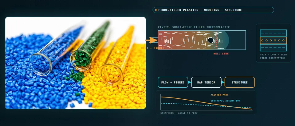
Fibre orientation simulation predicts how glass or carbon fibres line up as a plastic fills and cools in the mould, then carries that orientation into the structural model, so stiffness, creep, crash and fatigue are computed for the part as moulded, not for a datasheet modulus. We build the chain around your mould-filling solver and FEA code, with a validation record and surrogates of stated range.
The bracket passes on the datasheet modulus. Then the first shots from the production tool deflect more than the model said and a clip cracks along a line across its middle. Gate position and wall thickness were frozen with the tool, so every answer now costs steel and a slipped approval date. Auenhammer and colleagues (2024) note that in automotive development fibre orientation is commonly not considered and pseudo-isotropic models are used; Primetzhofer and colleagues (2019) describe fatigue design that assumed the worst orientation for the whole part, which gives away lightweight potential and cannot optimise the injection point.
What does fibre orientation simulation have to predict?
Four things: where the melt goes, how fibres align on the way, what cooling does to the shape, and what the finished wall can carry. A rigid fibre of aspect ratio r in a Newtonian flow rotates by Jeffery’s equation. Written for the orientation tensor A = ⟨p⊗p⟩, with Folgar and Tucker’s rotary diffusion for fibre contacts, it reads DA/Dt = W·A − A·W + ξ(D·A + A·D − 2A4:D) + 2CIγ̇(I − 3A). D and W are the symmetric and antisymmetric parts of the velocity gradient, ξ = (r2 − 1)/(r2 + 1), γ̇ the shear rate, and the fourth-order tensor A4 needs a closure.
The tensor is symmetric with unit trace and non-negative eigenvalues: five numbers per point. Gajek, Schneider and Böhlke call it the typical output of commercial moulding simulation. Tools implement variants such as RSC or MDR, and Greif and Meyer use ARD-RSC; we calibrate the variant and its coefficient against measured orientation, not a table.
- Flow lays the fibres down. Near the wall the melt is sheared fastest, the velocity profile by the gate, and fibres rotate toward the flow. At the advancing front, fountain flow carries material from the centre out to the wall, the curved arrows and travelling dots, where it freezes.
- Skin, shell and core. A thin skin freezes against the cold wall with irregular fibres. The shell, the thickest layer, is aligned with the flow, the long dashes. The core between the shells is off-axis; where the flow spreads out it lies across the flow, drawn end-on as circles. Layer thicknesses change with the part and the process window.
- Orientation is solved, not assumed. Each fibre rotates in the velocity gradient, and contacts between fibres add rotary diffusion, set by the Folgar-Tucker coefficient. The result is carried as a second-order tensor A, drawn as an ellipse. The fourth-order tensor in the equation needs a closure approximation, and variants such as RSC and ARD-RSC modify the rotation and diffusion terms. The variant and its coefficient are calibration targets.
- One averaged layer hides the shell. The curve is the simulated alignment through the wall: lower at the skin, high in the shell, lowest in the core. The dashed line is what a single through-thickness average keeps. Bending weights the outer layers most, so one average misstates flexure and local stress.
- Weld lines break the alignment. Where two fronts meet, the alignment is disrupted, the scattered ticks along the dashed line. Bonding across the joint is poor and voids and surface V-notches add to the loss. The weld position comes from the filling run; its strength comes from coupons cut with a controlled weld.
- Check the profile against the part. The dots with error bars stand for a measured profile from a section or CT scan. The pulsing ring marks a point where model and measurement disagree, the cue to revisit the process parameters or the orientation model. We tune them until the profile agrees at several locations, with one location held back.
The wall is layered. Auenhammer and colleagues describe an off-axis core, a shell layer predominantly along the flow and a thin skin from thermal shock at the cold wall; the shell is thickest. Primetzhofer and colleagues add that solidification at the wall leaves an irregularly oriented layer near the surface.
The filling run is itself a model: Auenhammer and colleagues name pressure and temperature progression, humidity and mould wear as sources of inaccuracy, and Primetzhofer and colleagues advise a CT comparison and tuning of process parameters.
How is fibre orientation mapped into the structural model?
The filling mesh is built for flow, the structural mesh for stress, so the field is transferred, and Primetzhofer and colleagues warn that the transfer can add deviations.
Tensors, not directions. A fibre and its reverse are the same fibre, so averaging directions cancels them, as Auenhammer and colleagues point out. Tensors average cleanly, and we test trace, symmetry and eigenvalues after every transfer.
Layers through the thickness. Automotive models usually represent mouldings by shell elements of 2 to 4 mm, say Auenhammer and colleagues, who map CT orientations onto five integration layers. The reason is flexure: the bending stiffness of a layered wall, D11 = ⅓ΣQ11,k(zk3 − zk−13), weights outer layers by z3, so one averaged tensor misplaces it.
Axes and stiffness. Eigenvectors become material axes, eigenvalues the degree of anisotropy, and a closure with mean-field homogenisation gives the stiffness, which Greif and Meyer pair with the IBOF closure. A material per point needs a user subroutine, as in the Abaqus runs of Gajek and colleagues; Wittemann and colleagues cluster the eigenvalues into 30 orthotropic materials and call fibre length crucial, asking for length distributions in the homogenisation.
- Process mesh: a tensor per cell. The filling run reports an orientation tensor in every cell, layered through the wall: irregular in the skin, flat and aligned in the shell, small and round in the core. It is a fine mesh built for flow and cooling, not for stress.
- Map the tensor, not a direction. Many fine cells collapse into a few layers of one structural element, the converging paths. A fibre direction p and its opposite −p are the same fibre, so directions cannot be averaged; tensors can. After mapping, each tensor is tested: trace one, symmetric, no negative eigenvalue.
- Structural element: layered points. Each integration layer holds its own tensor. The eigenvectors become local material axes and the eigenvalues say how anisotropic the layer is. Either a material per point is evaluated in a user subroutine or the eigenvalues are clustered into a limited set of material definitions.
- Stiffness depends on direction and layer. A closure and a homogenisation turn each tensor into a stiffness. The shell ellipse is stiff along the flow, the core ellipse across it, and the two fade in turn. The dashed circle is the isotropic datasheet material: one stiffness in every direction.
- The matrix is a state, not a constant. Temperature, absorbed moisture and loading rate or time move the matrix, so the properties come as ranges, the bars, with a fitted value, the fixed dot, for each condition you design for. Coupons along and across the flow set them.
- A surrogate answers inside its range. Designed runs over gate position, wall thickness and fibre content fill the dashed box. A query inside it is answered quickly; one outside, the pulsing dot, goes to the full process-to-structure model.
It matters. Gajek and colleagues mapped a filling result for a polyamide quadcopter arm onto an Abaqus mesh: under the same 80 N load the predicted deflection was 6.13 mm with a homogeneous isotropic orientation and 3.99 mm with the mapped one, a model-to-model comparison, not a test, and stress concentrations near the weld lines appeared only in the mapped model.
Why do weld lines and warpage need their own treatment?
Weld lines form where melt fronts meet, behind inserts or between gates. Nabergoj, Urevc and Halilovič (2025) list reduced molecular interdiffusion, voids, surface notches and disrupted fibre alignment, cite properties up to 50% below the base material, and note that commercial packages often use empirical weakening factors calibrated per geometry and process window. Their model adds initial damage to the weld, calibrated across the weld in glass-filled polyamide 66 and validated along it. We take the position from the filling run, the strength from coupons.
Warpage is a different mechanism. Greif and Meyer (2026) trace it to local variation in shrinkage plus anisotropy: stresses build while the part is held in the mould and release after ejection, and because warpage is non-local, shrinkage at one point can deform the whole part. A phenolic warpage chain by Wittemann and colleagues states its absolute values are not validated for lack of data. We rank gate and cooling variants with such a chain and tie the level to the shrinkage of your shots.
How do creep, rate, moisture and fatigue change the answer?
The matrix is soft and time-dependent. Pastukhov, Kanters and Engels (2021) model short-glass-fibre polyamide 6 with a viscoplastic law: Hill’s equivalent stress carries the load angle to the fibres, an apparent-temperature shift with a Ree-Eyring formulation carries temperature and humidity, and moisture-driven glass-transition depression sets the anisotropic kinetics. Tests therefore run along and across the flow at the conditioning states, temperatures and loading rates of service.
In fatigue, Primetzhofer and colleagues scale master S/N curves along and across the fibres with the first eigenvalue of the mapped tensor and correct node by node for notch, mean stress and temperature. In crash, explicit solvers such as LS-DYNA and Abaqus carry the orientation into an anisotropic, rate-dependent law whose failure strain depends on element size. See our composites fatigue and crash test simulation pages and a crash model you can trust.
Which model answers which design question?
| Question | Model chain | Reports | Limit to state |
|---|---|---|---|
| Where do weld lines fall? | Filling model over gate, runner and wall variants | Fronts, weld positions, tensors | Process window; check on sections or CT |
| Stiff enough? Which modes? | Mapped orientation, closure, homogenised stiffness, linear FEA | Deflection, frequencies per gate option | Closure, fibre length, conditioning state |
| Will it creep or relax? | Mapped orientation, viscoelastic or viscoplastic matrix | Deformation against time, temperature, humidity | Creep data along and across the flow |
| Crash response and fracture? | Explicit FEA, anisotropic rate-dependent law | Force-displacement, crack location | Failure tied to element size, weld, rate |
| Where does it fail in fatigue? | Local S/N on mapped orientation, notch, mean stress | Damage per node | Master curves, weld knock-down from coupons |
| Will it warp? | Process residual-stress and warpage model | Out-of-plane deflection | Non-local; matrix model; measured shrinkage |
| Which gate, wall, fibre content? | Surrogate over designed runs | Maps with ranges | Sampled range only; gate to full model |
A mapped orientation field is not a qualified part
Where does AI help fibre-filled plastics design, and where does it not?
- Surrogates over gate, wall and fibre content. Greif and Meyer trained neural networks on more than 600 simulated geometries and report a mean relative warpage error below 1% against the conventional simulation at six times the speed, with lower accuracy for very thin or lever-shaped parts. Their ground truth is simulated; real scans are not yet available in quantity.
- Tensor-safe outputs. They predict eigenvalues and eigenvectors, because six raw components can give non-physical stiffness. We build ours the same way.
- Micromechanics at every point. Gajek and colleagues use deep material networks, identified from linear-elastic microstructure runs, as surrogates across the orientation space.
- Calibration. Fitting the diffusion coefficient to CT profiles and weld damage to coupons, with the physics kept.
AI adds no data: creep, humidity, rate and weld strength still come from tests, and it does not extrapolate; we state the range and send cases outside it to the full model. See our surrogate modelling, hybrid physics-AI and uncertainty quantification pages and the articles on surrogate models and validating them.
From one moulded part to a workflow your team keeps
The return comes when your engineers push the next part or gate option through the same chain.
- Physics model. CFD and FEA set up once, as templates: geometry clean-up, mesh, solver settings and post-processing that every later run reuses.
- Validation. Mesh and time-step studies, and comparison with tests or full-scale data, so the model's uncertainty is known before it is trusted.
- Automated runs. Scripted runs over the parameters and operating conditions that matter, on your hardware or in the cloud.
- AI surrogate. A machine-learning model trained on those runs answers in seconds and says how sure it is; low-confidence questions go back to the solver.
- Decision tool. Optimisation, trade-off charts or operating guidance, in a form your engineers and operators use every day.
- Field data. Test, trial and monitoring data flow back to recalibrate the model, so it improves with every project instead of being rebuilt.
- A parametric filling template in your solver: gate, wall thickness, fibre content and process settings as parameters.
- A hand-over contract: tensors by layer in a versioned, tested file, with trace, symmetry and eigenvalue checks on every transfer.
- A material-card library, each card carrying its conditioning state, temperature, rate range and the coupons behind it.
- A validation record: orientation profiles from sections or CT, deflection or modal data from your shots, tolerances set before the run.
- A weld-line procedure: position from the filling run, a knock-down fitted on coupons and validated along the weld.
- A surrogate with a stated range and a gate to the full model.
- Handover and training: our training and software development services.
How credible is a fibre orientation result?
Verification is convergence and arithmetic: elements and layers through the wall, closure choice and the mapping checks. Validation uses data you hold or can make: orientation profiles from sections or CT, deflection or modal data on shots, coupons along and across the flow, one case kept back. Uncertainty is sampled over process window, conditioning state and material scatter; the answer is a range with ranked contributors. For the scale choice behind it, see composite modelling scales.
Questions engineers ask about fibre orientation simulation
Why not use the datasheet modulus for a glass-filled part?
How many layers through the thickness do I need?
Do I need moulded-in stress in the structural model?
Can simulation give the weld-line strength?
Does it replace sample shots and testing?
If a gate decision, a tool freeze or a stiffness, crash or durability approval is waiting on this, send us the part CAD with the gate options, the material grade and its conditioning state, any deflection or modal data from your shots, and sections or CT of a real part. We reply with the chain we would set up, the validation we would run and what a surrogate over gate, wall thickness and fibre content could cover. Start with a conversation, or see our plastic materials page.