Braided composite simulation from mandrel braid angle to progressive tube crush
The drawing says ±45°, the mandrel tapers, and the next lot of tubes crushes differently from the first. Process, unit-cell and crush models show which angle, yarn geometry or erosion setting is responsible.
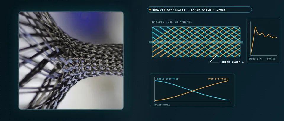
Braided composite simulation predicts the braid angle a machine lays down on your mandrel, the stiffness and torsion that angle gives a tube, and how the tube crushes progressively under load. We build it as a repeatable chain around your existing solver, with a validation record and a surrogate of stated range, so more of a braid-angle and layer decision is made before tubes are braided, cured and crushed.
The drawing says ±45°. The braider was set for it at the narrow end of a tapered mandrel and nobody has measured what the wide end received. The first crush tubes run a steady plateau; the next lot buckles from the same trigger. Each tube is a braiding run, a cure and a destroyed specimen, and a crash-structure release waits on a handful of them. Goldberg and colleagues (NASA Glenn and the University of Akron, 2012) wrote that impact simulation of triaxially braided carbon composites was limited by inadequate material data and a lack of validated models.
What does braided composite simulation have to predict?
Three models in a chain. The process model turns machine settings and mandrel geometry into a local angle, cover and thickness map. The unit-cell model turns that map into stiffness, strength and a damage sequence. The structural model predicts the tube’s stiffness, torsion and crush.
For a cylindrical mandrel the angle follows tan θ = ωR/v, with ω the carrier speed, R the mandrel radius and v the take-up speed. Bruyneel and colleagues (NAFEMS France, 2022) note that it holds only for cylinders and ignores transients, so on a taper at fixed speeds the angle changes along the part. Du-type differential equations cover variable circular sections in seconds, a kinematic projection onto a meshed mandrel covers any shape in a minute to an hour, and a beam-element finite element model adds friction at hours to days.
- Carriers and take-up set the angle. Carriers circle the ring in both directions while the mandrel is pulled along its axis. For a cylindrical mandrel the deposition angle follows tan θ = ωR/v, with ω the carrier speed, R the mandrel radius and v the take-up speed, as Bruyneel and colleagues write it. The angle is measured from the axis.
- A taper changes the angle along the part. At fixed carrier and take-up speeds the yarns keep the same axial pitch, so a larger radius means a steeper helix: the narrow end carries a smaller angle than the wide end, the two marked crossings. Holding the angle means varying the take-up speed with the radius, and the formula itself holds only for a cylinder.
- The unit cell sets the knock-downs. In a triaxial braid the axial yarns run nearly straight while the bias yarns undulate over and under them, and the local fibre axis follows each path, the small arrows and the travelling dot. Undulation, matrix pockets and the local fibre fraction are what a laminate calculation on the nominal angle leaves out.
- Stiffness moves with angle, by direction. Laminate theory for a ± θ pair gives these trends: axial stiffness falls and hoop stiffness rises as the angle grows, while shear and torsion stiffness peak between the extremes. The cross-over and the peak depend on the ply and the braid fill, so we compute them for your material and do not read them from the drawing.
- Four ways to get the angle map. The cylinder formula is instant but limited to cylinders. Du-type differential equations handle variable circular sections in seconds. A kinematic projection onto a meshed mandrel handles any shape in minutes to an hour, and a beam-element finite element braiding model adds friction at hours to days, the timings Bruyneel and colleagues report. The bars grow with cost and generality.
- The measured angle corrects the map. Angles computed from machine settings are sensitive to measurement error and to improper settings, as a 2021 review of tubular braid-angle measurement notes. We take the angle measured on the as-braided mandrel, by image processing, as the input that overrides the programmed value before the map reaches the unit cell and the structural model.
How does braid angle change axial, hoop and torsional stiffness?
For a balanced ±θ layer pair, axial stiffness falls and hoop stiffness rises as the angle grows from the axis toward the hoop, and shear and torsion stiffness peak between, near 45° for a typical carbon ply. But the angle on the part is not the programmed one: Ghamkhar and colleagues (2021) review tubular braid-angle measurement and note that angles computed from machine settings are sensitive to measurement error and improper settings. We take the angle measured on the as-braided mandrel as the input.
How do you build a braided unit cell?
Bruyneel and colleagues build the cell in five steps: lenticular yarn cross-sections, a path per yarn (nearly straight for axial yarns, undulating for bias yarns), solid yarns swept along the paths, a matrix box merged with them, and a cut to cell size. Orthotropy axes follow the yarn path, and cohesive interfaces can let the cell delaminate.
Zhao and colleagues (2019) model the triaxial cell with a continuum damage model, crack-band regularisation and tow-to-tow cohesive zones. Their notched-coupon model, 208,000 solid and 29,412 cohesive elements, ran about 20 hours per job on a 24-core workstation in Abaqus Explicit. A cell model is a property and damage tool, not the crush model.
Why do standard coupons mislead for braided composites?
Goldberg and colleagues tested a [0°/±60°] triaxial carbon braid. In transverse tension the straight-sided coupon, based on ASTM D3039, failed from damage that began at the cut edge and ran along the bias yarns: 462.0 MPa for one resin against 813.6 MPa for a double-edge-notched coupon, which they caution still has stress concentrations and a biaxial state.
Zhao and colleagues, citing earlier work, describe the free-edge effect as an elastic consequence of terminated bias bundles, and their predicted strength changed with whether complete axial tows remained across a gauge two unit cells wide. A braid property belongs to a coupon geometry as well as a material, so we record unit-cell size against coupon width and add a tube test, where no yarn is cut.
How do you simulate progressive crush of a braided tube?
Progressive crush absorbs energy in sustained fracture at a moving front, and a trigger starts it. Farley and Jones (NASA TM-101634, 1989) chamfered the tube end so the section loaded first is small and failure begins there, and named four crushing modes: transverse shearing, brittle fracturing, lamina bending and local buckling. Specific energy absorption and crush force efficiency summarise the curve.
The trend with braid angle is not a rule. Szederkényi and Bulman (2025) report that Farley’s quasi-static [0/±θ] carbon-epoxy tubes absorbed less energy as θ grew, while dynamic tests by Schmueser and Wickliffe suggest energy may rise with larger off-axis angles. A triaxial braid belongs to that family, though those tubes were laminated. Rate, fibre, matrix and failure mode decide the direction.
- The trigger starts the crush at the end. A chamfer on the tube end reduces the cross-section loaded first, so failure starts there at a load below the one that would fail the whole tube, as Farley and Jones describe in NASA TM-101634. The pulse marks where damage begins. In a model the trigger geometry is part of the result: meshed differently, it changes the first peak.
- The crush front does the work. Behind the trigger the wall splits into fronds that splay outward and inward around a wedge of debris, while the braid below stays intact. Farley and Jones name four crushing modes: transverse shearing, brittle fracturing, lamina bending and local buckling; splaying fronds are lamina bending. Fibre fragmentation and matrix crushing absorb the energy.
- Two numbers from one curve. The trigger sets the initial peak and the plateau after it carries the energy, the shaded area. Specific energy absorption is that energy per unit mass of tube, and crush force efficiency is mean load over peak load. The oscillation is real and a modelling hazard, so we compare filtered curves and integrals, not single points.
- One knob can flip the mode. In a shell model the strain at which a fibre element is deleted decides the mode. In the laminated-tube study of Szederkényi and Bulman a low compressive value gave global buckling from premature deletion, and a value set too high deleted too few elements and made the run unstable. The usable window is found by calibration and mapped, not assumed.
- Eroded and softened elements. At the front, elements that reach the deletion strain are removed, and the neighbours of deleted elements have their stiffness reduced so the whole section does not load at once, the blinking and shaded cells. Mesh size, contact definition and the softening factor all move the predicted crush, so calibration and use share one mesh.
- Building blocks, fitted automatically. Coupon data give stiffness and strengths. A triggered element is where the damage parameters are fitted, by automated identification rather than trial and error, as Garg and colleagues describe. A tube and then the component are held out to check, and each rung is trusted only after the test data agree.
Shells, cohesive layers or yarns for braided crush?
A shell model with continuum damage and element erosion is the working tool for tubes and components. Goldberg and colleagues represent each triaxial unit cell by four parallel laminated shells in LS-DYNA, strengths backed out of coupon curves. It has no continuous off-axis fibres, and rate matters: preliminary analyses gave local strain rates up to 2,400 per second, and a rate-sensitive model changed the predicted damage pattern, with no test data to judge it.
For the crush itself the erosion settings decide. Szederkényi and Bulman calibrated an LS-DYNA shell model of a 38 mm inner-diameter laminated tube to within 1% of the absorbed energy yet overestimated peak load by 9.2%. A low compressive erosion strain gave global buckling and a high one an unstable run, and they dropped cohesive layers as too many parameters. Garg and colleagues (2020) found that shell plus cohesive elements captured delamination but took 65 minutes per calibration iteration against 5, so they recommend shells for industry. Their material was a carbon twill, not a braid.
We set up a building-block ladder of coupon, triggered flat element, tube and component. Damage parameters are fitted by automated identification, 50 iterations of about five minutes each in Garg and colleagues’ shell model, not by trial and error; one tube is held out and the mesh is fixed between calibration and use. Energy-balance and mass-scaling checks follow our article on a crash model you can trust; the choice of scale is in our article on composite modelling scale.
Which braid question needs which model?
| Question | Model | Reports | Limit to state |
|---|---|---|---|
| What angle does this mandrel get? | Kinematic or Du-type; beam FE for odd shapes | Angle, cover, thickness map | Transients; measured angle decides |
| What stiffness and torsion will the tube have? | Laminate theory on local angle plus cell knock-down | Axial, hoop, shear stiffness | Undulation, fibre fraction |
| Where does damage start in the yarns? | Mesoscale cell, damage, cohesive zones | Damage sequence in the cell | Hours per job; cell against coupon size |
| What does the tube absorb? | Calibrated shell model with erosion | Load–stroke, energy, efficiency | Erosion, softening, mesh, rate |
| Does the wall split between layers? | Stacked shells with cohesive layers | Splitting and frond shape | Run time, extra parameters |
| Which angle and layers? | Surrogate on designed runs | Trade-off map | Sampled range; gate to full model |
A calibrated crush model is not a qualified structure
Where does AI help braided tube design, and where does it not?
- Surrogates over braid angle, axial-yarn content, layers, taper and trigger. Trained on designed runs of the calibrated model, they return stiffness, peak load, efficiency and energy absorption inside a stated range, with a gate to the full model.
- Unit-cell sweeps as a property surface: costly cell runs over angle and fibre fill become a lookup the structural model reads from the angle map.
- Automated calibration of damage parameters to load–stroke curves, bounds and objective recorded.
- Optimisation under your constraints: peak-load limit, packaging and mass go in first, and the best candidates are re-run in the full model.
It does not replace the angle map, which kinematic and differential-equation models already give in seconds to an hour. It does not carry a surrogate across a mode change: global buckling against progressive crush is a discontinuity, so we classify the mode first, regress inside each mode and send cases near the boundary to the full model. Crush curves oscillate, so targets are integrals and filtered values, with replicate runs that perturb mesh and erosion settings to measure the noise. See our surrogate modelling, uncertainty quantification and generative design and optimisation pages, and our articles on surrogate models and validating them.
From one tube study to a workflow your team keeps
The return comes when your engineers run the next angle, taper or layer count through the same chain.
- Physics model. CFD and FEA set up once, as templates: geometry clean-up, mesh, solver settings and post-processing that every later run reuses.
- Validation. Mesh and time-step studies, and comparison with tests or full-scale data, so the model's uncertainty is known before it is trusted.
- Automated runs. Scripted runs over the parameters and operating conditions that matter, on your hardware or in the cloud.
- AI surrogate. A machine-learning model trained on those runs answers in seconds and says how sure it is; low-confidence questions go back to the solver.
- Decision tool. Optimisation, trade-off charts or operating guidance, in a form your engineers and operators use every day.
- Field data. Test, trial and monitoring data flow back to recalibrate the model, so it improves with every project instead of being rebuilt.
- A parametric mandrel-to-angle model for your braider and mandrel family, checked against measured angles.
- A unit-cell generator and property library, each property tagged with the coupon geometry it was calibrated on.
- A crush template in your explicit solver, Abaqus, LS-DYNA or RADIOSS: trigger, mesh, erosion, softening and contact settings in one versioned file.
- A validation record against load–stroke curves, frond photographs and tube mass, tolerances set before the run, one tube held back.
- A surrogate with a stated range and a gate to the full model.
- Handover and training, so your team runs and extends it: our training and software development services.
How credible is a braided crush result?
Verification is convergence and balance: mesh and time step, energy balance and added mass, the trigger meshed as built. Validation uses data you hold or can generate: load–stroke curves filtered the same way, frond photographs, the measured angle along the tube, one tube kept back. Uncertainty is sampled: angle and fibre fraction along the tube, erosion and softening settings, rate dependence and numerical noise. The answer is a band on peak load, mean load and energy with ranked contributors.
Questions engineers ask about braided composite simulation
What braid angle is best for a crash tube?
Can a braid be modelled as a laminate?
How wide should a braided coupon be?
Which solver handles braided crush?
Does simulation replace crush tests?
If a crash tube or another braided part is waiting on this, send us the braid definition (yarn counts, tow sizes, bias angle, carrier count, take-up speeds), the mandrel drawing, fibre and matrix, layers and trigger geometry, and any crush or torsion data you hold: load–stroke curves and measured braid angles. We reply with the model chain we would set up, the validation we would run and what a surrogate could cover. Start with a conversation, or see our braided composites page and the wider composite materials section.