Flexible multibody dynamics with FEA: component loads for stress and fatigue
Rigid-body joint forces miss load share, resonance and impact ringing. How Craig-Bampton flexible bodies, checked at every hand-off, carry bearing, joint and contact loads into stress and fatigue models for machinery and drive systems.
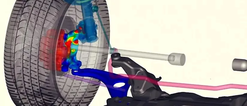
Flexible multibody dynamics simulates a machine in motion with some parts as elastic bodies, normally reduced from a finite element model by Craig-Bampton component mode synthesis, so the forces at bearings, joints and contacts include the flexibility of the parts that carry them. Coupled with FEA, the same run returns the stress history of each hot spot, ready for fatigue life.
The crack is at a bearing seat, a shaft shoulder or a carrier weld, and it shows up after the second season. The review asks what the loads were. Usually the answer is a rigid-body run: joint forces applied to a static model of the part with inertia relief, fixed before anyone knew whether the part would ring. Housing freeze waits for more rig hours, the lighter casting cannot be approved because nobody trusts the margin, and the warranty term stays conservative.
Why do rigid-body loads fail to predict stress in a flexible machine?
A rigid multibody model solves M(q) q″ + ΦqTλ = Q together with the constraints Φ(q, t) = 0. The multipliers λ are the joint reaction forces, and they come from the kinematics alone. A shaft on three bearings is statically indeterminate, so the split of load between its supports depends on whatever stiffness the joints were given, not on the shaft. A flexible body adds elastic coordinates: its deformation is u = Φη, mode shapes times modal coordinates η(t), solved together with the rigid motion.
Three effects follow, and each one changes the load that reaches fatigue. The load share between supports moves with the bending of the shaft. A force with content near an elastic mode of the part is amplified, and gear mesh, torque ripple and firing impulses all put energy there. And impact at a clearance excites a broad band of frequencies, so the peak the part sees is the impact plus the ringing that follows it. A rigid model has none of these, and the rigid assumption holds only while the loading has little content near the first elastic mode of every part in the load path.
How does Craig-Bampton reduction put a finite element part into a multibody model?
The degrees of freedom of the component are split into boundary dofs uB, where joints, bearings and contacts attach, and interior dofs uI. Spanos and Tsuha (NASA JPL, 1989) describe the Craig-Bampton mode set as the low-frequency fixed-interface normal modes augmented by static constraint modes. In matrix form, u = T [uB; η] with constraint modes Ψ = −KII−1KIB and the first k eigenvectors Φk of the interior with the boundary held. The reduced matrices are TTKT and TTMT, and a component with a full mesh becomes nB + k dofs.
Two properties make this the standard choice for machinery. The interface keeps physical coordinates, so a flexible body drops into the joint definitions of the rigid model, and a static load applied at the interface reproduces the full finite element response. The accuracy of the dynamics is then set mainly by k, which we choose against the frequency content of the loading and check by convergence. The boundary condition matters too: MacLean, Huynh and Quiocho (NASA Johnson Space Center, ASME 2007) note that the cantilever-type assumption common in manipulator formulations may not suffice for more general flexible systems, so we choose the interfaces and the mode set for the joint arrangement of your machine and test them.
- Full finite element component. The housing, shaft or bracket meshed in the finite element solver, with every node a degree of freedom. It is far too large to carry through thousands of time steps of a machine simulation.
- Interface nodes. Where joints, bearings, gear contacts and loads attach. The nodes around a bearing seat are tied to one master node, and these boundary coordinates are kept as they are, so the body connects to the rest of the model exactly as a rigid one would.
- Constraint modes. The static shape of the part when one interface coordinate is displaced and the others are held. Together they reproduce the response to any static load applied at the interface.
- Fixed-interface modes. The vibration of the interior with the interface held fixed. A low-frequency subset is kept; how many is decided by the frequency content of the loading and checked by convergence of the hot-spot stress.
- Reduced flexible body. In the multibody model the part has its interface coordinates plus a few modal coordinates. Its flexibility acts through the joints on the motion and on the loads of every neighbouring part.
- Stress recovery. After the run, the modal coordinates over time are multiplied by the stored stress field of each mode on the full mesh. The result is the stress history at any hot spot, ready for cycle counting.
How do bearing, joint and contact loads reach the fatigue model?
A flexible run returns three things. The first is the force and moment history at every interface, which can drive a local nonlinear finite element model of a bolted joint, a weld or a bearing seat. The second is the modal coordinates η(t), from which the stress at any point is recovered by superposition: σ(t) = Σi σi xi(t) over the interface and modal coordinates, with each σi the stress field of one mode, computed once in the finite element solver. A hot-spot history for a whole duty cycle is then a matrix product. The third is the contact state, which tells you where an impact happened and how hard.
The stress history becomes cycles by rainflow counting, one of the methods in ASTM E1049-85(2017), Standard Practices for Cycle Counting in Fatigue Analysis, which summarises irregular load histories by the number of cycles of each size, and cycles become damage with the material S-N data and the Palmgren-Miner sum, D = Σ ni/Ni. That is the work of our durability and fatigue life capability, and the link to it is the stress history, not a load scaled to a handbook factor. The hub names Ansys, Abaqus, Simpack and MSC Adams for coupled FEA and MBD with flexibility, and we build the chain around the solvers you already run.
- Drive and torque ripple. Gear mesh, firing or motor torque ripple enter as a time-varying excitation, with content across a range of frequencies that can meet the elastic modes of the parts downstream.
- Flexible shaft on bearings. The shaft bends, and the bearings are nonlinear springs. The split of load between supports follows from the bending and the bearing stiffness, which a rigid shaft cannot give.
- Clearance and contact. A pin or gear tooth crossing a gap closes it and strikes. The contact law and its stiffness decide the size of the impact, and the time step must resolve it.
- Force history. A rigid model returns a smooth pulse. A flexible model returns the same pulse with the ringing of the part's modes after the impact, and it is the ringing that adds cycles.
- Hot spot. The force history, scaled through stress modes, loads the bracket or housing. The fillet or seat with the highest stress range is where the fatigue life is decided.
- Cycle counting and damage. The stress history is reduced to cycles of each range by rainflow counting. Large ranges are rare, small ones frequent, and the damage sum weighs them with the material S-N data.
- Test correlation. Strain-gauge and vibration records from a rig or the field fit the bearing stiffness, clearance, contact stiffness and damping, and show which stage is wrong when the recovered stress does not agree with the gauge.
Where do clearance, contact and bearing loads really come from?
A pin in a bore with radial clearance is a contact problem: a force law such as F = Kδn plus a damping term, with n near 1.5 for a Hertzian point contact, switched on when the gap closes. It is stiff, so the time step must resolve the contact, and K is a property of the local geometry that a coarse reduced body does not contain. We take it from a local contact study or calibrate it. Impact then excites modes, so a rigid body shows a smooth pulse and a flexible one a peak followed by ringing, and fatigue counts the ringing.
Bearings are the same story with a spring in series. Their stiffness rises with load and depends on preload and clearance, and the shaft that sits in them bends. The force history that the bearing maker's life calculation needs comes out of that interaction, as does the misalignment at a gear mesh. Sills, Majed and Henkel (NASA, 2021) report the same logic at launch-vehicle scale: a flexible multibody approach lets contact and separation nonlinearities be treated in the coupled system instead of in separate local analyses.
How should a flexible multibody to FEA chain be checked?
- Rigid limit. Make the body very stiff: the reactions must return to those of the rigid model.
- Static check. Apply a static load at the interface to the reduced and the full model: displacement and hot-spot stress must agree.
- Mode convergence. Add fixed-interface modes until the hot-spot stress range stops changing for the highest-frequency loading in the duty cycle.
- Step convergence. Halve the time step: peak contact force and stress range must hold, or the contact is not resolved.
- Test correlation. Compare modal frequencies of the part or assembly with the reduced model, then the recovered stress with a strain-gauge record from a rig run.
| Load path | Use it when | It breaks when | Effort per design |
|---|---|---|---|
| Rigid multibody, joint forces to a static FE model with inertia relief | Parts are stiff against the loading and supports are statically determinate | Loading has content near a part mode, supports are indeterminate or impacts occur | Lowest |
| Flexible bodies by Craig-Bampton, stress recovered from modal coordinates | Elastic parts sit inside the load path and many duty cycles must be run | Plasticity or strong contact acts at the hot spot itself | Modes once, then fast runs |
| Flexible run, then interface loads into a local nonlinear FE model | The global response is linear but a bolt, weld, thread or seat behaves nonlinearly | The local model changes the global motion | Moderate |
| Full mesh inside the time loop (direct coupling) | Few load cases, and a local nonlinearity changes the global motion | Long histories and many duty cycles make it unaffordable | Highest |
Keep the hot spot away from the interface
Where does AI help flexible multibody simulation, and where does it not?
- A surrogate of hot-spot stress range and damage over bearing preload, clearance, mass and speed parameters, trained on a planned set of flexible runs, so a design sweep across duty cycles becomes affordable. See surrogate models for CFD and FEA.
- Calibration of bearing stiffness, clearance, contact stiffness and damping from accelerometer and strain-gauge records, a Bayesian fit that returns the parameters with their uncertainty, which then carries into the damage estimate.
- An anomaly gate on measured load cases, which flags a duty cycle outside the range the surrogate was trained on and sends it back to the solver. See AI surrogate models you can sign off.
Where it does not help: replacing the reduction itself, which is linear algebra whose error you can measure by adding modes; predicting an impact peak from rigid-body forces, which lack the timing and stiffness that set it; and extrapolating to a new bearing arrangement or part. Those go back to the physics.
From one load study to a flexible-body load path you keep
The return comes when your own team runs the next housing, shaft or duty cycle through the same checked chain.
- Physics model. CFD and FEA set up once, as templates: geometry clean-up, mesh, solver settings and post-processing that every later run reuses.
- Validation. Mesh and time-step studies, and comparison with tests or full-scale data, so the model's uncertainty is known before it is trusted.
- Automated runs. Scripted runs over the parameters and operating conditions that matter, on your hardware or in the cloud.
- AI surrogate. A machine-learning model trained on those runs answers in seconds and says how sure it is; low-confidence questions go back to the solver.
- Decision tool. Optimisation, trade-off charts or operating guidance, in a form your engineers and operators use every day.
- Field data. Test, trial and monitoring data flow back to recalibrate the model, so it improves with every project instead of being rebuilt.
- A library of flexible bodies: each housing, shaft, carrier and bracket reduced once in your existing solver, with its interface nodes, mode-count rule and stress modes stored, and regenerated by script when the geometry changes.
- A load-path template: duty cycle in, flexible multibody run, stress recovery, cycle counting and damage out, one command per operating case.
- A validation record: the five checks above for each variant, with the modal and strain-gauge data behind them.
- A surrogate with a stated range for hot-spot stress range and damage over the design and duty-cycle parameters, with a gate that returns out-of-range requests to the full chain.
- Handover and training, so your engineers add the next machine themselves. See our training and software development services.
Questions engineers ask about flexible multibody dynamics
What is flexible multibody dynamics?
What is the Craig-Bampton method and how many modes are enough?
Can I use rigid multibody joint forces for FEA fatigue?
How do you get stress from multibody results?
What do you need from us to start?
If a housing, shaft or bracket is cracking or is heavier than you can justify, send us the finite element model, the duty cycle, the bearing and joint data and any strain or vibration records. We will reply with which parts we would make flexible, where we would place the interfaces, which of the five checks we would run first and what the first stress history would let you decide. Start with a conversation. The wider multibody dynamics section and the machinery and mechanical drive systems page describe the capability.