Filtration CFD simulation for pressure drop, cake growth and filter cleaning
A skid is about to be frozen on a vendor's clean pressure drop for a datasheet duty, while your slurry blinds one cartridge early and cleaning never restores the baseline. We put flow split, cake growth, cleaning and wear on one validated chain, each model used within its range.
Filtration CFD simulation predicts how feed splits across the elements of a filter housing, how pressure drop climbs as cake builds and what cleaning gives back. Cartridge count, inlet layout and cleaning schedule can then be settled before the skid is built. No single model covers it: we chain a porous-media model of the housing, resolved particle runs for the cake and an erosion model for the walls. Each is fed with your media and slurry data, and we set the chain up around your existing solver, with its validation record.
The skid is about to be frozen, or a revamp pushes more throughput through housings sized for less. The vendor's guarantee rests on a clean pressure drop and a change-out interval for a datasheet duty, and your slurry is not the test dust. Then one cartridge blinds early, differential pressure creeps up because cleaning does not restore the baseline, and the inlet nozzle wears through before the elements do. The scope of ISO 11057:2011, a test for pulse-jet cleanable media, says its results are not intended to predict the absolute performance of full-scale filter facilities.
What does filtration CFD simulation have to resolve in a filter housing?
Parallel elements share the feed in inverse proportion to their resistance, and the header adds its own pressure variation. Park and colleagues (2021) measured the split in a ten-module water-treatment header and explained it with CFD. The last branch took about three times the flow of the first, because the pressure difference across the modules rose toward the end. The split moves as cake builds, since Bächler, Meyer and Dittler (2024) note that the flow divides by the current resistance of each element.
Each element enters the model as a porous zone: −∇p = (μ/K)u + βρ|u|u, Darcy's linear term plus Forchheimer's inertial one. K and β come from the supplier's pressure-versus-flow data at your viscosity, anisotropic for a pleat pack. It returns each element's flow share and the total pressure drop, not the flow inside a pleat. A steady RANS model with a two-equation closure covers the nozzle jet and header. We refine the mesh until the flow shares and the total pressure drop stop moving.
The pleat pack is where a porous zone is least honest. Teng, Shi and Zhu (2022) treat the V-shaped pleat corner as non-permeable because it carries so little flow, and the dead area grows as cake collects there. Their dust-loading model matched measured pressure drop on hand-made 140 mm test filters with a relative mean deviation of 3.68% for V-shaped and 4.82% for U-shaped pleats. That is a statement about those filters, not yours. We resolve a representative pleat and hand the housing an effective permeability and area.
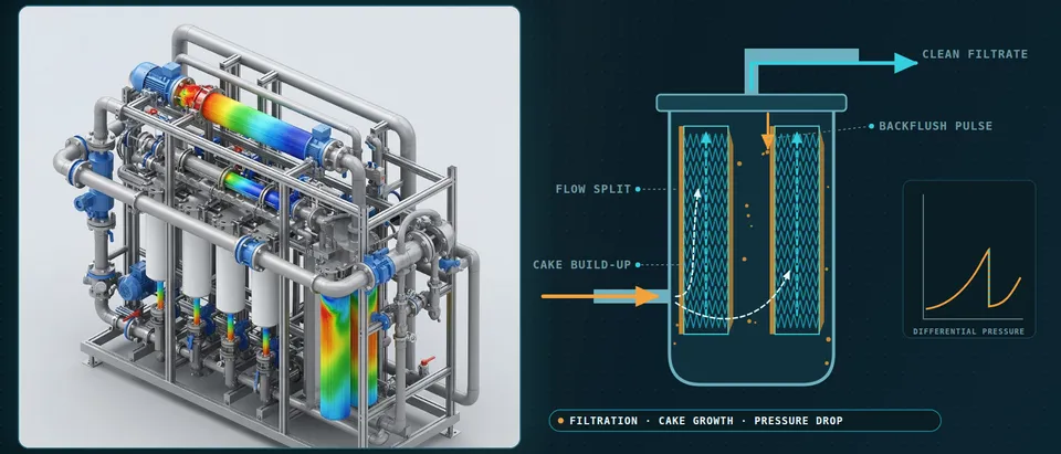
- Inlet and header set the split. Parallel elements share the feed in inverse proportion to their resistance, and the header adds a pressure variation of its own. In one operating water-treatment header, measured and simulated, the last of ten branches took about three times the flow of the first. Which element is favoured depends on nozzle, header and element resistance, so the split is computed, not assumed.
- Each element is a porous zone. The pleated element enters the housing model as a porous region: Darcy's linear term plus Forchheimer's inertial term, with permeability and inertial coefficient taken from the supplier's pressure-versus-flow data at your viscosity. The shading shows each element's share of the flow. The model returns that share and the pressure drop, not the flow inside a pleat.
- Pleat roots are dead zones. Inside the pack, dirty-side channels narrow toward the core. Flow enters over the upper faces and the root sees little: in an open-access dust-loading study the pleat corner was treated as non-permeable, and the ineffective area grew as cake collected there. A resolved pleat supplies the effective permeability and area to the housing model.
- Cake grows where the flow goes. Deposited solids add a cake resistance in series with the medium, so the elements and faces that take more flow load faster and the split shifts as cake builds. The housing model adds the cake resistance to the local porous resistance at each time step, with the specific cake resistance taken from filtration tests on your slurry.
- Wear where particles cannot turn. Particles with enough inertia keep their path where the fluid turns: at the dead end of a header, a nozzle exit or a baffle edge. Lagrangian tracks give the impact speed and angle on each wall face, and an empirical erosion law, calibrated on measured wall loss, ranks the hot spots.
- Clean side, cores and tubesheet. Clean fluid collects through the element cores into the plenum, and the differential pressure across element, cage and tubesheet is what FEA needs. At the pressure limit and during cleaning, CFD pressure is mapped to the structure to check the margin around the supplier's collapse rating.
How are cake growth and particle deposition simulated?
Pressure drop is the sum of the medium, the cake and the transition layer where the first particles block pores, as Puderbach, Schmidt and Antonyuk (2021) set out. Their equation v = Δp / μ(RC + RM) is what every model must reproduce. Plotted as t/V against V, a constant-pressure test gives the specific cake resistance from the slope and the medium resistance from the intercept.
At sample scale the cake is a particle problem. Puderbach and colleagues couple a lattice-Boltzmann flow solver to the discrete element method, resolving the fluid around every particle. The test used silica glass spheres of 63–100 µm on a 32 µm woven wire cloth at 1,000 Pa. The simulated specific cake resistance, 7.8×10¹⁰ m−2, matched the measured 7.7×10¹⁰. The run covered only the start of filtration, 161 particles, with the fitted line extended to the measured filtrate volume, and fluid-particle forces were accurate at 40 voxels per particle diameter. Unresolved CFD-DEM needs a drag correlation for the swarm effect.
A housing holds far too many particles to resolve, so the sample result becomes a closure. Resolved runs and filtration tests on your slurry fix the specific cake resistance and the interference resistance. Housing-scale Euler-Lagrange tracks then deliver the deposited mass per area, which adds resistance to the local porous zone at each time step. Cohesive, sticky and compressible cakes need measured properties: the same paper calls stick-on-contact permissible for gas filtration but needing a sticking probability for liquids.
Why does differential pressure follow a sawtooth, and what does cleaning restore?
For one element, Δp = (Kmedium + Kcake·W)·w, and cleaning resets the deposited mass W. Bächler and colleagues show that reset is an idealisation. The medium resistance fitting their nine-bag baghouse measurements changed with cleaning interval and tank pressure, which they tie to the residual pressure drop of patchy cleaning. The cleanable-media test, DIN ISO 11057 in their account, assumes a fully regenerated filter area at constant volume flow.
The paper sums up the interval as a three-way trade. Longer intervals lower average emissions at the cost of higher differential pressure. Shorter ones lower pressure drop but use more compressed air and raise emissions, since particles penetrate only directly after regeneration. That is a baghouse result; for a liquid backflush your own data set the trade. CFD adds the transient reverse flow and where it reaches. Whether a cake detaches is a material property, so cleaning efficiency is a measured input and residual cake carries into the next cycle.
- Cake growth is the ramp. For one element the pressure drop is the medium resistance plus the cake resistance times the deposited mass per area, all times the face velocity. As cake builds the pressure drop climbs, and a compressible cake curves the ramp upward. The slope depends on the slurry, which is why cake resistance is measured, not assumed.
- Cleaning resets only part of it. A pulse or backflush sends a reverse flow through the medium and lifts cake away, so the pressure drop falls almost at once. A transient run shows how the reverse flow spreads along and across the elements; whether a given cake detaches is a material property, taken as a cleaning efficiency measured on your tests.
- The baseline creeps up. Patchy cleaning leaves cake on part of the media. In a nine-bag pulse-jet baghouse study the medium resistance that fitted the measurements changed with cleaning interval and tank pressure, so each cycle starts higher than the last. The model carries residual cake from one cycle into the next instead of resetting to a clean element.
- Breakthrough after cleaning. For pulse-jet cleaned gas filters, the same paper states that particles penetrate the medium only directly after a regeneration, before a new cake forms, and an approximately fixed amount escapes per event. For a liquid duty, check the equivalent in your own solids data before assuming it away.
- The interval is a trade-off. That paper sums up the trade: longer intervals lower average emissions at the cost of higher differential pressure; shorter intervals lower the pressure drop but use more compressed air and raise emissions. The glyph and bars alternate between the two. For a liquid backflush the same trade is set by your own test data.
- The limit comes from the element. The pressure drop at which you must clean or change out is set by the element's rating, the pump or fan and the process, not by the model. We take that limit from your data and the supplier's, and use the pressure-drop-versus-time curve to show how many cycles remain before you reach it.
Where does separator erosion come from, and how far can the model be trusted?
In cyclones, hydrocyclones, strainers and inlet nozzles the recipe is Lagrangian. Flow and particle tracks give impact speed and angle on each wall face, and an empirical erosion law turns them into wall loss. Mahmoudi and colleagues (2025) follow it for particles in water through two elbows in series and validate it against experiment. They use empirical angle-dependent restitution and an erosion model chosen for its handling of particle shape. Upstream geometry changed the hot spot. Peak erosion in the second elbow at a 24-diameter connecting length was about 15% of that at three, so the inlet piping belongs in the model.
Trust is bounded by the coefficients. The poster of Karimi and colleagues (2020) notes that erosion models were mainly built on data at much higher velocities and lower temperatures than the concentrating-solar particle systems it studies. The first term of the model it prints scales with impact speed to the power 2.41, so a 10% speed error becomes about 26% (1.12.41). We calibrate on your measured wall loss and report ranked hot spots and sensitivities, not a service life.
Which filtration question needs which model?
| Question | Model | What it reports | Data you supply |
|---|---|---|---|
| Flow split and header layout | Steady RANS, porous elements | Flow share, total pressure drop | Element pressure-flow curve |
| Pleat-pack pressure drop | Resolved pleat | Effective permeability and area | Pleat pitch, height, media thickness |
| Cake resistance | Resolved CFD-DEM sample | Specific and interference resistance | Particle size distribution |
| Cake growth in the housing | Euler-Lagrange plus cake resistance | Deposition map, pressure drop against time | Cake resistance from tests |
| Pulse or backflush | Transient reverse flow | Reverse-flow distribution | Cleaning efficiency from tests |
| Wall erosion | Euler-Lagrange plus erosion law | Ranked impact hot spots | Wear survey |
| Element, cage, housing load | FEA with CFD pressure | Stress and margin | Supplier collapse rating |
How do pressure loads reach the cage and the housing?
At the pressure limit and in a pulse, CFD pressure goes to FEA through a conservative transfer. The loads go to the cage, tubesheet, nozzle reinforcements and the wall left after erosion, and pulse cycles are a fatigue duty (see our durability and fatigue life and fluid-structure interaction pages). The collapse rating is the supplier's; FEA shows the margin around it. Combustible dust needs a separate venting study.
A simulated pressure drop is not a performance guarantee
Where does AI help filtration design, and where does it not?
- Inlet layout and cartridge count. A designed set of housing runs trains a surrogate of each element's flow share and the total pressure drop. An optimiser searches the layouts, and anything outside the sampled range returns to full CFD.
- Calibration. An inverse fit of cake resistance, residual baseline and cleaning efficiency to your differential-pressure history returns a range and flags drift in media or slurry.
- Change-out forecasts. The filter equation carries the trend, a learned correction carries what it misses, and the physics stays the fallback.
It does not replace the cake test on a new slurry, repair wrong media data or extrapolate: Bächler and colleagues fitted the medium resistance with a logarithmic function of cycle time and warn that higher-degree polynomials fit better inside the data and make extrapolation much harder. A surrogate inherits the closure errors of its training runs. See surrogate models for CFD and FEA, surrogate validation and our surrogate modelling, hybrid physics-AI and uncertainty quantification pages.
From one housing study to a filtration workflow you keep
The return comes when the next housing, slurry or cleaning strategy goes through the same chain.
- Physics model. CFD and FEA set up once, as templates: geometry clean-up, mesh, solver settings and post-processing that every later run reuses.
- Validation. Mesh and time-step studies, and comparison with tests or full-scale data, so the model's uncertainty is known before it is trusted.
- Automated runs. Scripted runs over the parameters and operating conditions that matter, on your hardware or in the cloud.
- AI surrogate. A machine-learning model trained on those runs answers in seconds and says how sure it is; low-confidence questions go back to the solver.
- Decision tool. Optimisation, trade-off charts or operating guidance, in a form your engineers and operators use every day.
- Field data. Test, trial and monitoring data flow back to recalibrate the model, so it improves with every project instead of being rebuilt.
- A parametric housing template in your existing solver: nozzle, header and element count as parameters, with turbulence, mesh and porous-zone choices on record.
- An element data loader that turns supplier pressure-versus-flow data into porous coefficients, with the viscosity range stated.
- A cake and cleaning calibration from your filtration tests and plant trend.
- An erosion post-processor that ranks wall-loss hot spots, tied to your wear survey.
- A validation record against a flow-split measurement and a pressure-drop trend, tolerances set first.
- A surrogate with a stated range and a gate to the full model outside it.
- Handover and training, so your team runs and extends it. See our training and software development services.
Questions engineers ask about filtration CFD
How accurate is CFD for filter pressure drop?
Can CFD predict the change-out interval?
Why do parallel cartridges load unevenly?
What data do I need from the filter supplier?
If a skid freeze, revamp or element change-out shutdown is waiting on a filtration CFD simulation, send us the housing and nozzle drawings and the element data sheet. Add the slurry properties with particle size distribution, a differential-pressure trend over several cleaning cycles and any inlet wear survey. We reply with the model chain we would set up, the filtration tests the cake model needs, its validation record and what a surrogate could cover. Start with a conversation, or read our filtration system design page and multiphase methods page.