Stirred tank CFD for agitator design, blend time and scale-up
The pilot vessel blended in moments and the plant vessel does not, while an agitator order, a shutdown window or a vendor guarantee waits on the answer. Stirred tank CFD, with a checked rotation model, tracer set-up and shear metric, puts power, blend time and scale-up on one validated chain.
Stirred tank CFD predicts how an agitator moves liquid: the power it draws, how fast a feed blends, where fluid hangs back and how hard the impeller shears it, so a design can be judged before a pilot run. It is only as good as its rotation model and tracer set-up: in one published study, the size of the rotating zone in a steady model moved predicted mixing time by up to a factor of three. We build that chain around your solver, with its checks on record.
The pilot vessel blended the feed in moments. The plant vessel still shows a gradient at the sample port, the batch is on hold, and nobody can say whether the agitator or the scale-up is wrong. An agitator order, a vendor guarantee, a revamp with a new impeller or drive and a shutdown window that opens once all wait on it. A power-per-volume rule set the speed; what it did to blend time and blade-tip shear is unknown.
What does stirred tank CFD have to resolve?
The impeller turns shaft power into a discharge jet and turbulence, baffles stop the liquid from merely rotating, and the flow closes into circulation loops. It draws P = NpρN3D5 at Re = ρND2/μ, and once the flow is fully turbulent Np stops changing with speed; Wagner and colleagues (2026) find it near 5.5 for a Rushton-type turbine in a baffled tank, Re from 5×10⁴ to 1.25×10⁵.
Blend time follows: for fixed geometry it is a nearly fixed number of revolutions, about 20 for 90% homogeneity in their lattice-Boltzmann simulations, independent of Reynolds number. Buoyancy breaks it: from a stratified fill of two liquids the same tank at Re = 125,000 needed about 79 revolutions at a Richardson number of 10, and in their Ri = 12 case the lighter liquid was sealed off from the stirrer's power input.
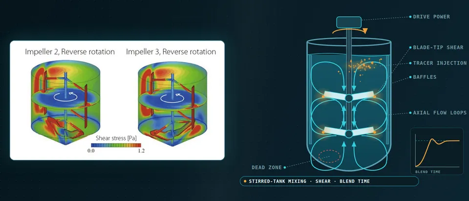
- Power and discharge jet. Shaft torque times rotation rate is the power. In dimensionless form P = Np ρ N³ D⁵, and in fully turbulent flow Np is constant for a given geometry, so power rises with the cube of speed. A radial turbine discharges a jet that splits into an upper and a lower loop.
- Trailing vortices and tip shear. Behind every blade a vortex pair forms, and the highest dissipation in the tank sits in this very small volume (lower chart), far above the tank average. A cell, crystal or drop meets it once per circulation, so its exposure history matters more than the peak or the mean.
- Baffles. Wall plates stop the liquid from simply rotating with the impeller, turn the swirl into axial flow and raise the power draw. They also shelter stagnant pockets, and they force a blade-baffle interaction that a steady model sees at one blade angle only.
- Circulation loops. A radial turbine drives two loops, with the return flow along the shaft. How often a fluid element comes back to the impeller sets how fast a feed spreads: for a given geometry in fully turbulent flow the blend time is a nearly fixed number of impeller revolutions.
- Tracer feed and probe response. A tracer fed at one point is carried round the loops and a probe records it at another. Blend time is the time after which the signal stays within a band, commonly 5%, of its final value. Feed and probe positions both change the answer, so a result must state both.
- Slow regions, or dead zones. Fluid under the free surface and below the impeller exchanges with the loops slowly, and a feed that lands there blends last. Where the slow regions sit depends on liquid level, clearance, baffles and impeller type. A tracer run shows them as the last cells to reach the band, which the mean velocity does not.
MRF, sliding mesh or LES: which impeller model?
A steady multiple-reference-frame (MRF) model solves a zone around the blades in a rotating frame and the rest in a stationary one: cheap, with the zone size left to the user. Reid and colleagues (2025) compared five zone diameters, 1.10 to 1.93 impeller diameters, in the Rushton-turbine tank of Wu and Patterson (1989). Velocity profiles agreed with the measurements for every zone. The smallest zone gave a power number more than 12% lower, larger zones grew an artificial band of turbulent kinetic energy at the zone boundary, and a passive-scalar run changed mixing time by up to a factor of three.
Velocity passed the check; the quantity the plant cares about moved. We sweep zone size and blade angle as standard and report the spread.
A sliding mesh rotates the impeller mesh through the baffle mesh in time. It resolves blade passage, trailing vortices and blade–baffle interaction and makes torque a time series, with a time step that resolves the passage. Large-eddy simulation adds the large eddies, and with it uncovered a low-frequency, precessing flow in a Rushton-turbine tank (Hartmann, Derksen and Van den Akker, 2004) whose period spans many blade passages: a steady run cannot show it.
- Rotating-zone interface. A steady multiple-reference-frame (MRF) model solves a zone around the blades in a rotating frame and the rest of the tank in a stationary one. The zone size is a user choice. In a published Rushton-turbine study, larger zones, closer to the baffles, grew an artificial band of turbulent kinetic energy at the interface and shortened the predicted mixing time.
- One blade angle. The steady model freezes the blades at a single angle to the baffles, so it returns one value at a monitor point and no time history. Mean velocity barely changed with blade angle in the same study; turbulence profiles did.
- Sliding mesh. The inner mesh rotates through the stationary baffle mesh, so blade passage, trailing vortices and the blade-baffle interaction are resolved and torque becomes a time series. The price is a time step that resolves the passage and many revolutions to average.
- Blade-passing signal. A monitored velocity or torque ripples at the blade-passing frequency. That ripple is the fluctuating load on the shaft and part of the fluctuating shear, and a steady run returns neither.
- Slow wander (macro-instability). Large-eddy simulation of a Rushton-turbine tank has uncovered a low-frequency, precessing flow structure whose period spans many blade passages. It modulates the bulk flow and the kinetic energy of the fluctuations, so the averaging window must cover many such periods.
- Resolved eddies. Large-eddy simulation resolves the energy-containing eddies and models only the small ones, so turbulence and dissipation are computed rather than assumed by a closure. Its cost makes it a reference or a final check, not the loop for a design sweep.
Verification differs by output. In the Reid study power number moved 0.9% between 3.3 and 5.8 million cells while turbulent kinetic energy was still not converged, and k-ε over-predicted turbulence where k-ω SST captured the double peak. The measurements carry their own uncertainty, within 4% for velocity and 15% for turbulent kinetic energy; Wagner and colleagues put the numerical uncertainty of power number at 2.39% from a three-grid study following ASME V&V 20.
How is blend time predicted, and where are the dead zones?
Blend time comes from a passive tracer: scalar transport on a frozen flow field with a turbulent Schmidt number, which Reid notes ranges from 0.3 to 1 across studies, and blend time taken as the moment a probe stays within 5% of its final value. In that paper one probe read 19.5 s with the smallest rotating zone and 9.5 s with the largest.
So we report a field, not a probe: when each cell last leaves the band. The last cells to arrive are the dead zones, and they move with feed point, liquid level, clearance and baffles. A feed lighter or heavier than the bulk behaves like the stratified cases above.
How much shear does an impeller create?
Peak shear sits in a small volume behind the blades and the tank average is far lower; what a cell, crystal or drop experiences is neither but its history of passes through the loops. In a CHO cell culture study (Kenmoku and colleagues, 2025) average shear stress correlated best with titer loss among ten CFD parameters (ρ = −0.64, against −0.58 for the maximum), and the authors cite work pointing to the frequency of passage through high-stress regions.
Criteria also disagree on one field. In a 3 L single-use bioreactor (Kreitmayer and colleagues, 2022) hydrodynamic stress, √(ρμε), judged the highest speed below critical, while the Kolmogorov length, (ν3/ε)1/4, flagged a few computational cells behind the blades at the size of a mammalian cell; the authors note no experimental evidence relates it to viability. For crystallising and emulsifying duties we carry the same exposure statistics and ask which one your product responds to.
Why does stirred tank scale-up fail?
With geometric similarity, fully turbulent flow, constant Np and a blend time fixed in revolutions, scale-up is algebra, and no choice satisfies everything. For a diameter factor λ:
| Held constant | Speed | Tip speed | Power per volume | Blend time |
|---|---|---|---|---|
| Power per volume | λ−2/3 | λ1/3 | same | λ2/3 |
| Tip speed | λ−1 | same | λ−1 | λ |
| Speed | same | λ | λ2 | same |
| Reynolds number | λ−2 | λ−1 | λ−4 | λ2 |
Constant power per volume keeps average dissipation but raises tip speed and lengthens blending; whether that matters depends on whether your product responds to the average or the local maximum. Real tanks are not geometrically similar anyway: level, feed point and catalogue impeller sizes differ. We simulate pilot and plant as built, validate on the pilot and compare the same metrics at both scales. The scope of ASME V&V 20-2009 is accuracy at validation points where the experiment is simulated, with extrapolation left to engineering judgment: a pilot validation carries to the plant only inside its stated range.
Sparged gas and suspended solids add phases and need a multiphase model with its own validation; see our multiphase flow page.
Which stirred tank question needs which model?
| Question | Model | What it reports | Limit to state |
|---|---|---|---|
| Power draw | Steady MRF, torque on blades | Power number, mean flow | Zone size swept; not from dissipation |
| Blend time, dead zones | Tracer on frozen or transient flow | Local mixing-time field | Feed, probe, Schmidt number |
| Shear: sensitive, crystallising, emulsifying | Sliding mesh or LES, particle tracks | Dissipation, exposure history | Criterion set per duty |
| Fluctuating shaft loads | Sliding mesh | Torque, side-force series | Many revolutions |
| Pilot to plant | Same model, both vessels as built | Same metrics at both scales | Inside validated range |
| Sparged gas, suspended solids | Multiphase model | Hold-up, suspension | Own validation |
How do agitator loads reach the FEA model?
The surface forces that give power also load the shaft: integrated about the axis they are torque, and their lateral resultant is the bending load. A steady run gives the mean at one blade angle, a transient run the part that fluctuates at blade-passing frequency. We map pressure and shear to the structural mesh with a conservative transfer, check stress, fatigue and natural frequencies in FEA, and close the loop if shaft deflection changes the flow. See our fluid-structure interaction and durability and fatigue pages.
A predicted blend time is not a performance guarantee
Where does AI help stirred tank design, and where does it not?
- Design sweeps. A surrogate over impeller diameter, speed and off-bottom clearance returns power, torque, blend time and shear exposure in seconds, for an optimiser.
- Calibration. Pilot data fit zone size and Schmidt number to a range, not a point.
Naderibeni, Wu and Tax (2026) trained neural surrogates on steady RANS runs of an industrial multi-impeller vessel over speed and liquid height: error fell steadily with more operating conditions, with diminishing returns, physics constraints helped most when data were scarce, interpolation was reasonable, and feeding learned fields back into a tracer solver proved numerically fragile. They say uncertainty quantification would help most in extrapolation. So we surrogate the scalar outputs a decision uses and send anything outside the sampled range to the full model.
A surrogate reproduces its training data, zone artefacts included, only faster; it cannot repair a closure, extrapolate to a new rheology or gas load, or replace a tracer test. See our surrogate modelling, uncertainty quantification and optimisation pages and surrogate validation.
From one tank study to a mixing workflow you keep
The return comes when your engineers put the next vessel, impeller or duty through the same chain.
- Physics model. CFD and FEA set up once, as templates: geometry clean-up, mesh, solver settings and post-processing that every later run reuses.
- Validation. Mesh and time-step studies, and comparison with tests or full-scale data, so the model's uncertainty is known before it is trusted.
- Automated runs. Scripted runs over the parameters and operating conditions that matter, on your hardware or in the cloud.
- AI surrogate. A machine-learning model trained on those runs answers in seconds and says how sure it is; low-confidence questions go back to the solver.
- Decision tool. Optimisation, trade-off charts or operating guidance, in a form your engineers and operators use every day.
- Field data. Test, trial and monitoring data flow back to recalibrate the model, so it improves with every project instead of being rebuilt.
- A parametric tank template in your existing solver: impeller, clearance, baffles, level, speed and feed point as parameters, with one record of rotation-model, zone, closure and time-step settings.
- A sensitivity sweep of zone size, blade angle, mesh and Schmidt number with every case, so the spread is reported beside the result.
- Post-processors for power from torque (integrating dissipation under-predicts it in RANS), blend-time and dead-zone fields, shear exposure and an FEA load hand-over.
- A validation record against an open Rushton-turbine data set and your pilot data, tolerances set before the run.
- A surrogate with a stated range and a gate to the full model.
- Handover and training, so your team runs and extends it. See our training and software development services.
Questions engineers ask about stirred tank CFD
How long does a stirred tank take to blend?
What is the difference between MRF and a sliding mesh?
Is constant power per volume the right way to scale up?
Can CFD guarantee the power or blend time of an agitator?
If an agitator order, a scale-up or a revamp is waiting on a blend-time, power or shear answer, send us the vessel and impeller drawings, the fluids and operating window, the duty, any pilot power or tracer data and the decision date. We reply with the model, validation and sweep we would set up for each question, what a surrogate could cover and what we need from you. Start with a conversation, or read our mixer design page and consulting service.