Hall thruster simulation for ionisation, wall erosion and plume design
The facility slot is booked and the magnetic circuit is waiting to be frozen. Hall thruster simulation ranks topologies, flows and voltages before the wear test, around an electron-transport closure that is calibrated to measurements and checked against vacuum-facility data.
Hall thruster simulation couples the magnetic circuit, ionisation zone, electron transport across the field, walls and plume, so a magnetic topology, flow or voltage can be compared on a computer before it is built and wear-tested. Its hard limit is that no first-principles model yet predicts how electrons cross the field, so we calibrate that closure to measurements, bound it with a validation record and check it against facility data, around your existing solver.
The facility slot is booked and the design review wants the magnetic circuit frozen. A new pole piece means another wear test, and the answer you need, which surface erodes first and how wide the plume reaches, arrives thousands of hours later. Kaganovich and colleagues state it in their 2020 review of E×B discharges: thruster development rests on a semi-empirical approach with long, expensive lifetime tests, on the order of 10,000 hours. Simulation does not remove that test; it decides which candidates reach it and how its result is read.
What makes Hall thruster simulation hard?
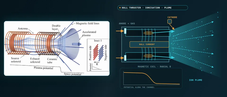
An axial electric field accelerates ions in the annular channel while a radial magnetic field, strong enough to magnetise electrons and too weak to bend ions, holds the electrons back. They drift azimuthally at E/B, a closed Hall current, and ionise the propellant. For singly charged ions falling through V, vi = √(2eV/mi), thrust is F ≈ ṁivi and efficiency is η = F2/(2ṁP).
The scales are wide: a Debye length of about 50 µm, breathing oscillations below 100 kHz that couple plasma and neutral density through ionisation, and electron-drift waves above 1 MHz with wavelengths below 1 mm. Collisions alone leave electrons far too little cross-field mobility, classically falling as 1/B2. The measured discharge needs more, and the cause is not yet predicted from first principles, so every model carries an empirical or kinetic stand-in.
- Gas in, ionisation zone. Neutral propellant enters at the anode and is ionised where electron density and energy peak. Neutrals deplete and refill, so plasma and neutral densities oscillate together: the breathing mode, below 100 kHz. A zero-dimensional model predicts it where its one-dimensional equivalent shows none, and it is sensitive to electron mobility, so the transport model decides whether a simulated discharge breathes.
- Radial field, closed Hall current. The magnetic circuit sets a radial field across the channel. Electrons are magnetised and drift azimuthally at E/B in a closed ring; ions, with a far larger Larmor radius, are not. Field strength, curvature and the position of its peak are what a sweep changes, and the bowed lines near the exit are the shielding topology.
- Electrons hop across the field. Electrons from the cathode must cross field lines to reach the anode. Classical collisions give too little mobility, so fluid codes add an anomalous collision frequency, the cyclotron frequency times a function f_a(r,z) fitted to plasma measurements. No validated first-principles closure exists yet, so this is the calibration knob.
- Where the potential falls. Unmagnetised ions are accelerated by the axial field, which is strong where the electron current is held back. Thrust follows ion flux and speed. The curve is qualitative: where the fall sits shifts with field topology, flow, voltage and facility pressure, and the simulation has to follow it.
- Walls and shielding. Sheaths set the ion energy at the walls and so the erosion, and secondary electron emission from the wall material adds near-wall conductivity. Shielded topologies hold plasma potential high and electron temperature low near the walls so ions arrive with little energy. The flashing dots mark the bombardment that erosion estimates are built from.
- End view: the ring that rotates. Along the axis the Hall current is a ring of azimuthal drift. A spoke rotates around it and short waves grow on the drift. Azimuthal PIC resolves them; a two-dimensional model overstates the instability, with cross-field mobility more than five times a three-dimensional one.
- What the solver carries. A practical axisymmetric model carries multi-fluid ions, an empirical anomalous collision frequency with a stated fitted range, and a wall and sheath treatment. PIC runs on small domains test its assumptions. Each part keeps its calibration data and its limit.
How is a Hall thruster simulated, and where does each model fail?
The workhorse is a two-dimensional axisymmetric (r–z) code on a field-aligned mesh with ions as several fluids, because one fluid would convect slow near-plume ions at the fast ions' mean velocity and give erroneously low density outside the beam (Kamhawi and colleagues). Its electron collision frequency is νa = fa(r,z)ωce, with fa guided by plasma measurements. Early hybrid codes assumed Bohm 1/B scaling, which could not explain the plasma inside the channel; the empirical function gave some of the closest agreement with time-averaged measurements, without statistical noise, though fluid ions miss the ion velocity distribution (Kaganovich and colleagues).
PIC with Monte Carlo collisions resolves the instability behind the transport, at a price: for a three-dimensional channel and near plume the same review estimates 103 nodes per coordinate, picosecond steps, 108 steps, over 103 particles per cell and about 1021 operations. Two-dimensional models cost less but overstate the instability, with cross-field mobility more than five times the three-dimensional estimates. So PIC answers physics questions on small domains and the calibrated fluid model answers design questions; we verify PIC runs against the benchmark on which seven independent codes agreed within 5% (Charoy and colleagues).
How do you keep anomalous electron transport repeatable?
We treat fa(r,z) as data with provenance: parameterised, fitted to laser-induced fluorescence (LIF) ion velocities or probe profiles and mapped against the operating window, so the post-processor flags runs outside it. Machine learning can automate the fit: Jorns used it to replace the human iteration that finds the collision frequency from measurements, as Kaganovich and colleagues report.
Injected probes perturb the plasma and must be avoided when validating thruster codes, so the record names the diagnostic behind every data point. And a transport assumption carried across topologies is a hypothesis: the topology study below assumed the collision frequency follows the peak field as it retracts, and LIF showed the acceleration zone moving upstream, but not one-to-one with it.
What does Hall thruster erosion simulation tell you?
Sheaths set the ion energy at the walls, and secondary electron emission from the wall material adds near-wall conductivity that can cut thrust. Magnetic shielding holds plasma potential high and electron temperature low near the channel surfaces; on a 6 kW laboratory thruster it cut erosion by a few orders of magnitude. Wear then moved to the front pole covers: a 3,000-hour wear test of a 12.5 kW unit gave peak rates of 140 and 80 µm per thousand hours, inner and outer cover, at 300 V and 6.25 kW. Kamhawi and colleagues simulated four new topologies, oscillations included: channel erosion peaked near 100 µm per thousand hours, about two orders below the unshielded thruster, and computed thrust stayed within 5% of the measured baseline. Simulation ranks candidates and the wear test confirms them; an erosion rate is an estimate, not a service life.
Why does the vacuum chamber change thruster test results?
Dankanich and colleagues record that background pressure is a primary facility effect: performance is mainly affected by ingested gas, lifetime by the ion flux that erodes surfaces, the far-field plume by the plasma the facility creates. No universal theory predicts it, and their recommended practice sets limits tightening from 3×10⁻⁵ Torr for performance and 1.3×10⁻⁵ for the near-field plume to 5×10⁻⁶ for life tests, as an initial position.
Limits are thruster-specific. Huang and colleagues saw thrust, efficiency and ion current density of a 12.5 kW thruster turn nonlinear above about 10-5 Torr, and advise testing at several pressures below it and extrapolating linearly to zero; plume data accurate to 10% may need 10-6 Torr, so they calibrate a plume model instead. Snyder and colleagues measured 2–4% more thrust from an SPT-140 at 10 µTorr than at its lowest pressure above 1 kW. Chamber walls also supply material: in a hybrid-PIC study (Choi and colleagues) facility-wall carbon dominated redeposition on the anode and channel wall in the model.
So the facility is part of our model, with background gas, backsputter and chamber connection as inputs. The validation record logs the pressure behind every data point, and an in-orbit estimate is a calibrated extrapolation, not a raw test number.
- Primary ions at large angles. Most beam ions go forward, but the plume characterisation of a 12.5 kW magnetically shielded thruster detected primary ions at 90 degrees polar angle. With enough flux they erode spacecraft surfaces and complicate where thrusters can sit, so plume divergence is a design output.
- Charge exchange. A fast ion takes an electron from a slow neutral: a fast neutral leaves and a slow ion is born. Slow ions are pushed by local fields sideways and backward, toward surfaces behind the exit plane. Plume models keep fast and slow ion populations apart and link them only through charge exchange.
- Background gas and pumping. Residual gas is ingested at the exit and changes the ionisation. Pressure is not uniform: lower near the pumps and higher near the plume, so where the gauge sits matters. Performance, life and far-field plume data respond differently, and no universal a priori theory predicts the effect for every thruster.
- Backsputter. The beam erodes the target and material returns to the thruster. In a hybrid-PIC study of a thruster with graphite pole covers, facility-wall carbon dominated redeposition on the anode and channel wall in the model, so a wear test carries the facility's signature unless it is modelled.
- The pressure sweep. Below a limit the response is linear, above it nonlinear. For one 12.5 kW thruster, thrust, efficiency and ion current density turned nonlinear above about 10⁻⁵ Torr, so data at several pressures below the limit are extrapolated linearly to zero. The limit is thruster-specific, not a constant.
- From near field to surfaces. The calibrated near-field solution feeds a plume model and then erosion and deposition on spacecraft surfaces. Plume measurements to 10% accuracy may need pressures a facility cannot reach, so the plume model is calibrated on data at several pressures, not trusted from one.
What does the plume do to the spacecraft?
The plume characterisation of that 12.5 kW thruster detected primary ions at 90° polar angles; with enough flux they erode spacecraft surfaces and complicate placement. Charge exchange adds a slow population: the plume model links fast and slow ion groups only through it. We hand the near-field solution to your spacecraft-integration tools for erosion and contamination studies, with our thermal analysis and aerospace simulation services alongside.
How does a helicon or magnetic-nozzle thruster change the model?
Electrodeless thrusters have no Hall current or channel wall. A wave solver (our electromagnetic multiphysics work) supplies the power that ionises and heats the plasma, and a divergent magnetic nozzle accelerates it through an ambipolar field whose potential falls along the nozzle. Ions detach from the field lines, which sets divergence, and the electrons' diamagnetic current pushes on the coils as magnetic thrust. The plasma is near-collisionless, so the fluid closure is open and kinetic models complement fluid ones; facility effects are more acute (Kaganovich and colleagues).
Which Hall thruster question needs which model?
| Question | Model | Reports | Limit to state |
|---|---|---|---|
| Discharge position and thrust against topology, flow, voltage | r–z fluid or hybrid, multi-fluid ions | Potential, ion flux, thrust | Transport fitted per thruster |
| Instabilities and transport | Axial–azimuthal PIC-MCC | Spectrum, mobility | 2D overstates mobility |
| Oscillation response | Time-resolved hybrid | Frequency, amplitude trends | Sensitive to mobility |
| Wall and pole-cover erosion | Fluid or hybrid with sheath, yield data | Erosion rate by surface | Estimate, not a life |
| Plume on spacecraft surfaces | Plume model with charge exchange | Current density, ion energy by angle | Calibrated at several pressures |
| Zero-pressure performance | Facility model, multi-pressure extrapolation | Estimate with its band | Linear below a limit |
| Sweeps over topology, flow, voltage | Surrogate on designed runs | Thrust, current, erosion maps | Stated range, gate |
A simulated erosion rate or thrust is not a qualification
Where does AI help Hall thruster design, and where does it not?
- Surrogates over the design window. Trained on designed runs of the calibrated model over topology, flow and voltage, they return thrust, current, an erosion index and plume current density in seconds, within a stated range and with a gate to the full model. Operating mode is classified first, since a 12.5 kW thruster turned more oscillatory from about 450 V.
- Transport calibration. An inverse fit to LIF and probe data returns ranges of fa.
It does not predict anomalous transport from first principles, carry a surrogate across topology families or facility pressures, or stand in for the wear test. See our hybrid physics-AI, surrogate modelling and uncertainty quantification pages and our articles on surrogate models and validating them.
From one thruster study to a design workflow you keep
The return comes when your team can run the next topology or throttle point through the same chain.
- Physics model. CFD and FEA set up once, as templates: geometry clean-up, mesh, solver settings and post-processing that every later run reuses.
- Validation. Mesh and time-step studies, and comparison with tests or full-scale data, so the model's uncertainty is known before it is trusted.
- Automated runs. Scripted runs over the parameters and operating conditions that matter, on your hardware or in the cloud.
- AI surrogate. A machine-learning model trained on those runs answers in seconds and says how sure it is; low-confidence questions go back to the solver.
- Decision tool. Optimisation, trade-off charts or operating guidance, in a form your engineers and operators use every day.
- Field data. Test, trial and monitoring data flow back to recalibrate the model, so it improves with every project instead of being rebuilt.
- A parametric thruster model in your existing solver: geometry, field map, flow and voltage as parameters, one template.
- A transport library with fitted ranges, data sources and an out-of-range map.
- A facility module with background gas, pressure and backsputter.
- A validation record against thrust, discharge-current spectrum, ion velocity and wear profiles, tolerances set first.
- Erosion and plume post-processors exporting to your spacecraft tools.
- A surrogate with a stated range and a gate to the full model.
- Handover and training, so your team runs and extends it. See our training, software development and consulting services.
Questions engineers ask about Hall thruster simulation
Can simulation predict Hall thruster lifetime?
Why is anomalous electron transport modelled empirically?
Fluid, hybrid or PIC for a Hall thruster?
How low must chamber pressure be to trust thruster data?
Does this cover helicon and magnetic-nozzle thrusters?
If a topology freeze, throttle table or facility test plan is waiting on this, send us the thruster geometry and magnetic circuit or field map, the operating window, what you have measured (thrust, current waveforms, probe or LIF data, wear data) and the facility pressure and pumping set-up. We reply with the model chain we would set up, the validation we would run against your data and what a surrogate could cover. Start with a conversation, or see our plasma thruster page and the plasma simulation hub.