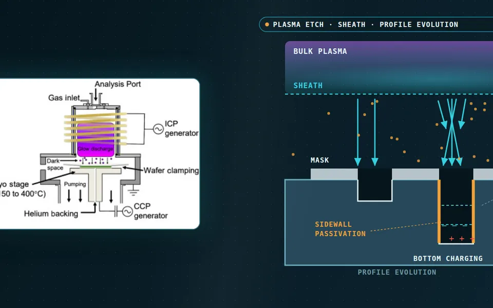
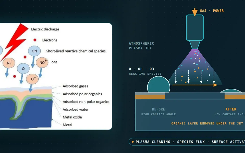
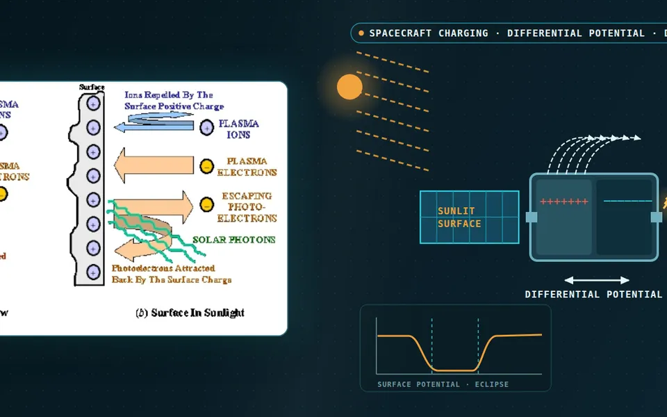
Magnetron sputtering simulation for racetrack, target life and film uniformity
The new magnet pack erodes the target where the drawing did not say, the film is thick in the middle and the reactive recipe jumps. A chain of magnetostatic, PIC-MCC, rarefied-gas and surface-balance models shows which link is responsible, and what to measure to settle it.
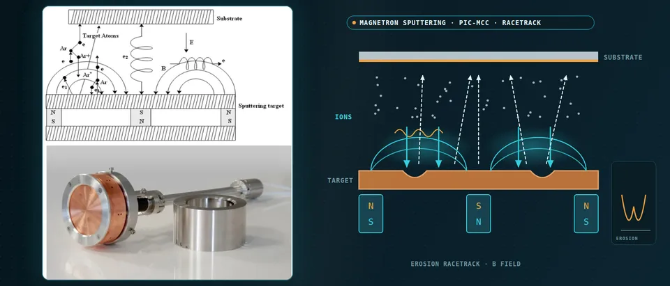
Magnetron sputtering simulation follows one chain: the magnet array sets the field, the field traps the electrons that form the racetrack, the racetrack decides where the target erodes, and the erosion sets the flux that reaches the substrate. We model each link with the method its physics needs, calibrate it on your coater and leave it with your team as a workflow.
The new cathode is on the coater with a new magnet pack. The first target comes out with its groove in the wrong place, the film is thick in the middle, and the reactive recipe that held last week jumps between metallic and poisoned mode. Pack release, target-change interval and recipe transfer wait on it, and the usual answer is another target. Walton and colleagues at Lawrence Livermore call the lack of knowledge of internal process conditions a key challenge in magnetron sputtering, and note that film stress depends sensitively on the energies and angles of arriving atoms.
Why is magnetron sputtering simulation hard?
Only the electrons are magnetised: their gyroradius rL = mv⊥/(eB) is small against the source, the ions' is not. Electrons drift at E/B and, on a planar source, circle back on themselves; that closed drift is the racetrack, where ionisation, ion bombardment and erosion concentrate and which limits target utilisation. The sheath is millimetres thick, about 3 mm in the balanced DC example of Zheng and colleagues, on a source far larger, and an explicit PIC code must resolve the Debye length λD = (ε0kTe/ne2)1/2 and the electron plasma period. Fluid plasma models lose accuracy at low pressure and strong field, as the same authors note. And the neutral gas is not at rest: the sputtered flux heats and thins it.
How do you simulate the magnet array and the racetrack?
We start from the pack in electromagnetic FEA (see our electromagnetic multiphysics work), with the finite magnets resolved. Locker and Strauß, in a 2026 preprint, compare point dipoles with a field integrated over the finite magnets: the dipole version broadens the erosion band, while the finite-magnet field gives a groove whose width is close to the geometric estimate 2√(2reLRc), with reL the electron Larmor radius and Rc the field-line curvature radius at the target. They call the magnet geometry a first-order modelling choice and, lacking a field map, had to infer magnetisation from nominal remanence; a field map of your real pack fixes it in our model.
Balanced sources close the field lines on the cathode; unbalanced ones leave some open towards the substrate. Zheng and colleagues show that for a balanced DC source a 1d3v PIC-MCC run reproduces the density, potential profile and ionisation rate of the 2d3v run above the racetrack if its current density is the local racetrack value, 2 mA/cm2 against 0.2 nominal, though its voltage came out near −500 V against −420 V. We use 1D to screen balanced sources and 2D or 3D for unbalanced ones.
- Magnet pack and field. The north-south-north pack sends field lines up through the target and back. Where a line runs parallel to the surface, electrons are held and the racetrack forms. Balanced sources close the lines on the cathode; unbalanced ones leave some open towards the substrate. The finite magnets must be resolved, because a point-dipole field broadens the confinement, and the remanence is fixed on a measured field map.
- Trapped electrons and E×B drift. Electrons spiral along the lines with a small gyroradius and drift at E/B around the ring, out of the page on one side and into it on the other, while ions barely feel the field. Ionisation concentrates where electrons are held, shown as the glow. PIC-MCC follows these orbits and their collisions, so its time step and mesh must resolve the gyration, the Debye length and the plasma period, or use an implicit scheme.
- Sheath, ions and the supply. Argon ions fall through the cathode sheath almost straight onto the target. The supply and its series resistor decide where the discharge settles: the crossing of the load line with the discharge's own voltage-current curve, drawn on the right. The secondary-electron and electron-reflection coefficients that shape that curve are fitted to your measured curve.
- Erosion groove. Ion flux times sputter yield digs the groove under the glow; the dashed line is the original surface. As the groove deepens the target thins and the field and plasma shift, so one run on a fresh target is not the whole life. We run fresh, mid-life and late-life profiles and check them against a depth trace of your eroded target.
- Sputtered flux in hot, thin gas. Atoms leave with a Thompson energy distribution and a cosine angular law, then cross gas that their own momentum has heated and thinned: sparse dots inside the warm region, dense dots outside. Collisions there set the energy and angle that reach the substrate, so the gas is solved kinetically, not as a continuum at the set pressure.
- Film profile on the substrate. Each substrate point collects the flux integrated over its path past the source. The right panel contrasts a fixed substrate, with humps above the grooves in the drawing, with a moving one, which averages them flatter. One flux map per target state plus the substrate motion gives the thickness map without rerunning the plasma.
Why must the power supply sit inside a PIC-MCC model?
The cathode voltage is an outcome, not an input. With a supply and series resistor, Vext = U0 + RextIext, and the discharge settles where that load line crosses its own voltage-current curve. Bultinck and colleagues coupled such a circuit to a 2d3v PIC-MCC model of a circular planar magnetron. In their abnormal-glow case, at 1 Pa, the circuit model gave 0.43 A against 0.4 A measured; imposing the same cathode potential instead converged to 0.008 A, almost two orders too low, and in their normal-glow case the discharge went out. Secondary-electron emission and electron reflection at the cathode are fitted, not computed: they cite a shift of about 30 V in cathode potential when the reflection coefficient moves from 0 to 0.5. We fit both to your voltage-current curve at two or more pressures and carry their range into every result.
How do you model sputtered-atom transport and gas rarefaction?
Atoms leave the target with a Thompson energy distribution, f(E) ∝ E/(E + Eb)3 with Eb the surface binding energy, and a cosine angular law, the pairing Bobzin and colleagues suggest. For an industrial coater with two magnetron cathodes at about 0.5 Pa of argon they estimate a mean free path near 1.4 cm and a Knudsen number Kn = λ/L between 0.05 and 1.5. Navier-Stokes held only up to about Kn = 0.1: their fluid solution showed a large circulation around the substrate holders that their kinetic DSMC solution did not. We keep the gas kinetic, by DSMC or test-particle Monte Carlo, wherever Kn exceeds that bound.
The flux also reshapes the gas it crosses. Walton and colleagues cite up to about an 85% reduction of the background gas density at high current density; their DSMC run of a 4 A copper source in 1 Pa of argon heats the gas to about 1000 K on the axis and raises the pressure there by 40 to 50%, and agreed with probe data to within 10 to 40%, with further validation needed.
Reactive sputtering simulation: why does the process jump?
Reactive sputtering changes the target: compound forms on its surface and the sputter yield changes, typically dropping significantly for oxides, as Barynova notes. Gas-phase reactions are negligible, so the chemistry sits on the target, substrate and walls. Berg's balance: Qin = pS/kBT + αtF(1 − θt)At + αsF(1 − θs)As, reactive flow in equals pumping plus consumption on the uncovered target and collector. Gajdics and colleagues restate Berg's condition for hysteresis: somewhere the reactive flow needed falls as the pressure rises. There the operating point jumps, and sweeping the flow up and down traces different branches. In their RF alumina rig, without a magnetron, power and pumping speed shifted the loop; feedback control or superimposed low-frequency pulses stabilise the process. Our model carries your pumping speed, geometry and measured loops and returns the stable window and its margin, not a recipe; sticking coefficients and compound yields come from your sweeps.
- Gas in, pump out. Reactive gas enters at flow Q and leaves through the pump at speed S; whatever the pump does not remove is consumed on surfaces, which is the balance in the pill below. Pumping speed is a measured input of the model and it moves the whole hysteresis loop.
- Target coverage and yield. Gas arriving on the target forms compound, ion bombardment removes it, and the coverage is the balance of the two; the patches fade between the metallic and the poisoned state. The compound sputters at a lower yield, and for oxides typically a significantly lower one, so the deposition rate falls as coverage grows.
- Sputtered metal as a getter. Fresh metal arriving at the substrate and the walls binds reactive gas, a second sink in the balance beside the target. Dark dots are metal atoms and warm dots are reactive gas. In the classical Berg balance the target coverage and the collector coverage are both unknowns.
- The S-curve and its hysteresis. Steady states form an S. On the dashed middle branch the gas flow needed falls as the pressure rises and that state is unstable, so sweeping the flow up and then down follows two different branches with a jump at each fold. The travelling dot walks the loop; the pulsing rings mark the jumps.
- Pumping speed moves the loop. In an RF alumina rig without a magnetron, Gajdics and colleagues found that a lower pumping speed moved the loop to lower flow and a higher power moved it to higher flow. The dashed ghost loop shows such a shift. The model carries your pumping speed and power, so its loop can be compared with your measured up-and-down sweep.
- Holding the unstable branch. Feedback control holds a pressure or voltage setpoint by adjusting the flow, which can let a process run on the unstable middle branch between the jumps; superimposed low-frequency pulses are another route. The ring marks such a setpoint. The model shows where a setpoint is reachable and how much margin a recipe has; it does not replace the control tuning on your tool.
What changes in HiPIMS and pulsed sources?
HiPIMS adds ion return. Barynova's 2026 dissertation attributes the often lower HiPIMS deposition rate to back-attraction of film-forming species ionised near the target, and finds that the sputter yield dictates the back-attraction probability and the degree of gas rarefaction. Its ionisation-region model is a zero-dimensional balance whose free parameters, back-attraction probability and the share of discharge voltage across the ionisation region, are fitted to measured current and voltage with the ionised flux fraction as a constraint. Global models cannot represent spokes, ionisation zones travelling along the racetrack; those go to PIC.
Which magnetron sputtering question needs which model?
| Question | Model | Reports | Limit to state |
|---|---|---|---|
| Where is the racetrack? | Pack FEA; electron Monte Carlo or 2D PIC-MCC | Field map, groove width | Needs a measured field map |
| What voltage at this current? | PIC-MCC with the supply in the loop | Voltage-current curve, ion flux | Emission, reflection fitted |
| Where does the flux land? | Source terms; DSMC transport | Arrival flux, angle, energy | Cross-sections; Knudsen regime |
| Where does the reactive process jump? | Berg-type balance, measured pumping | Loop, stable window | Sticking, yields from sweeps |
| HiPIMS current and ionised fraction? | Global model; PIC for spokes | Pulse response, back-attraction | Fitted parameters; no spokes |
| Sweeps over magnet, pressure, power | Surrogate on designed runs | Maps with a gate | Stated range |
How do you predict film uniformity and target life?
Once the flux is known, uniformity is bookkeeping: the thickness at a point on a moving substrate is the deposition rate integrated over its path past the source, so one flux map per target state plus the substrate motion gives the thickness map without rerunning the plasma. The target state is the hard part: a closed-loop calculation that updates erosion, field, plasma and transport as the groove deepens is, as Locker and Strauß note, not yet routine. We stage it: fresh, mid-life and late-life groove profiles, each with its own field, discharge and flux map, checked against a depth trace of your eroded target and witness-coupon thickness maps.
A simulated racetrack is not a process release
Where does AI help magnetron sputtering design, and where not?
- Surrogates over the design space. Trained on designed runs of the chain over magnet position, pressure and power, a surrogate returns groove width and flux uniformity in seconds inside a stated range, with a gate to the full model outside it.
- Calibration. An inverse fit of emission, reflection and sticking parameters to measured voltage-current curves and hysteresis loops returns ranges, not single values.
- Regime guards. A classifier on the reactive map keeps a regressor from averaging across the jump between metallic and poisoned mode.
It does not repair a wrong cross-section set, remove PIC noise, interpolate across a hysteresis jump or stand in for the target-life test. See our pages on surrogate modelling, hybrid physics-AI, uncertainty quantification and optimisation, and our articles on surrogate models and validating them.
From one magnet study to a sputtering workflow you keep
The return comes when your engineers can put the next pack, target material or recipe through the same chain.
- Physics model. CFD and FEA set up once, as templates: geometry clean-up, mesh, solver settings and post-processing that every later run reuses.
- Validation. Mesh and time-step studies, and comparison with tests or full-scale data, so the model's uncertainty is known before it is trusted.
- Automated runs. Scripted runs over the parameters and operating conditions that matter, on your hardware or in the cloud.
- AI surrogate. A machine-learning model trained on those runs answers in seconds and says how sure it is; low-confidence questions go back to the solver.
- Decision tool. Optimisation, trade-off charts or operating guidance, in a form your engineers and operators use every day.
- Field data. Test, trial and monitoring data flow back to recalibrate the model, so it improves with every project instead of being rebuilt.
- A parametric source model of pack, target, shield and substrate path, in your existing solver, in commercial codes or in new subroutines, with thermal analysis of the cooled target.
- A calibration set: field map, voltage-current curves at two pressures, hysteresis sweep in both directions.
- A validation record: eroded-target depth trace and witness-coupon thickness maps, tolerances set before the run.
- A surrogate with a stated range and a gate to the full chain.
- Handover and training, so your team runs and extends it: see our training and software development services.
Questions engineers ask about magnetron sputtering simulation
Can simulation predict target erosion and utilisation?
Do I need PIC-MCC, or is a fluid model enough?
Why does my reactive hysteresis loop move with pumping speed?
Can it replace a coater trial or witness coupons?
If a pack release, a target-change interval or a recipe transfer is waiting on this, send us the pack drawing or field map, an eroded-target depth trace with its energy, voltage-current curves at two pressures, a reactive sweep in both flow directions and a substrate thickness map. We reply with the model chain we would set up, the validation we would run and what a surrogate could cover. Start with a conversation, or see our magnetron sputtering page or the plasma simulation hub.