Spacecraft charging simulation for differential charging, ESD and materials
A shaded dielectric beside a harness, a coating that has to stay conductive, an eclipse that moves every potential. Spacecraft charging simulation shows where surface differences approach the discharge thresholds, how a transient couples into electronics, and what the ground test must measure.
Spacecraft charging simulation predicts the potential each exterior surface reaches in a given plasma environment, the differences between surfaces and structure ground, and whether they approach the thresholds at which an electrostatic discharge (ESD) can occur. It lets a team compare coatings, grounding and geometry before the design is frozen and aim the ground test. We set it up around your existing solver, with material data held as ranges, a validation record and a surrogate of stated range.
The design review is next week. Blankets, coverglass and paint are chosen, a harness runs beside a shaded dielectric panel, and a worst-case hand estimate puts surface differences above the 400 V that NASA-HDBK-4002B, Mitigating In-Space Charging Effects, adopts as its threshold of concern. Each fix costs something: optical or thermal performance for a coating, mass for a bond, facility time for more testing, and all rest on emission data nobody measured on your lot. The handbook is blunt: neglecting charging has contributed significantly to the loss of spacecraft functions and, indeed, of the entire vehicle.
How does spacecraft charging simulation predict surface potential?
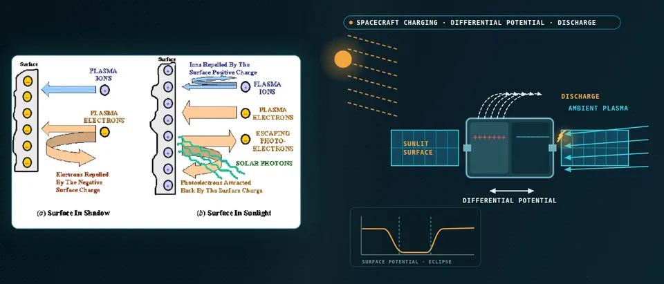
The physics is current balance. At equilibrium the currents a surface collects sum to zero: ambient electrons and ions, secondary and backscattered electrons, photoelectrons and any active source. Electrons are far more mobile than ions, so a surface in shadow charges negative until repelled electrons match the rest. The handbook gives milliseconds for the whole body and up to hours between surfaces.
Sunlight decides which surfaces matter. At geosynchronous orbit photoemission usually dominates, so sunlit surfaces sit a few volts positive of the plasma and structure is kept from charging strongly negative. The handbook's worst-case plasma (its 90th percentile) is a single Maxwellian: electrons at 12 keV and 1.12 cm−3, ions at 29.5 keV and 0.236 cm−3. The Debye length is then roughly 770 m, so GEO charging can be solved as an electrostatic field around the vehicle with particle trajectories, not a resolved sheath.
Eclipse changes the question: absolute potentials shift, and differential charging in eclipse builds slowly and depends on differences in secondary yield. With secondaries ignored, first order gives V ≈ −Te ln(Ie0/Ii0) (handbook Eq. 9), but secondary currents decide the real answer and Te must exceed a critical value, usually of order 1000 eV, before charging occurs.
- Sunlit surface. Photoelectrons leave the illuminated surface. At geosynchronous orbit the NASA handbook says this photoemission usually dominates, so sunlit surfaces sit a few volts positive of the plasma and structure ground is kept from charging strongly negative. The model needs the photoemission yield and the sun angle for every patch.
- Shaded dielectric. With no photoemission, plasma electrons, far more mobile than ions, drive a shaded dielectric strongly negative relative to space, to structure ground and to its sunlit neighbours. Most electrons are repelled and ions are drawn in. The difference between surfaces is the discharge risk, not the absolute potential.
- Current balance. At equilibrium the currents a surface collects sum to zero: ambient electrons and ions, secondary and backscattered electrons, photoelectrons and any active source such as a thruster. The model solves it for each surface and for the capacitive coupling between surfaces, which is where differences come from.
- Emission data. Secondary electrons released by impact set where the balance lands. Purvis found predicted equilibrium potential sensitive to essentially all the electron-yield parameters, and Lundgreen and Dennison describe wide measured ranges. We carry yields as ranges, with contamination and end-of-life cases, not single numbers.
- Orbit and eclipse. The handbook gives milliseconds for the whole body to reach equilibrium, seconds to minutes for isolated surfaces against ground and up to hours between surfaces. Eclipse entry and exit change absolute potentials; differences in eclipse build slowly and depend on secondary yield. The model runs the timeline, not one snapshot.
- First-order screen. In eclipse, ignoring secondary currents, the potential follows the electron temperature times the log of the electron-to-ion current ratio (handbook Eq. 9). The handbook cautions that secondary currents matter and that the temperature must exceed a critical value, usually of order 1000 eV, before charging occurs. We use it to sanity-check the full model, not as a result.
Why is differential charging, not absolute potential, the ESD risk?
Breakdown follows differences. The handbook quotes a rule of thumb that a dielectric surface more than about 500 V positive of an adjacent exposed conductor may break down, adopts a more conservative 400 V, and adds that a field above 2 × 10⁷ V/m at a dielectric-to-grounded-conductor interface may discharge. Edges, gaps and seams raise local fields and are not usually modelled; inspection finds what the model cannot.
What a discharge releases follows stored charge. The handbook adapts three classes from NASA-TP-2361: minor below 0.5 µC, moderate 0.5 to 2 µC, severe 2 to 10 µC. It calls computing the charge lost highly speculative and notes no generally accepted physics-based theory of dc breakdown exists. So we report potentials, fields, stored charge and energy (½CV²) against thresholds with the spread stated, never “will discharge”.
What does a design-grade charging model have to get right?
Model choice follows the question. Lumped-element models give each surface its own independent current input, so, the handbook notes, they tend to predict larger negative voltages than observed; three-dimensional codes capture how one area's charging changes the flux to others. The SPIS project describes hybrid, full-PIC and backtracking models in one 3D electrostatic solver.
Inputs decide the answer as much as the solver. Purvis found equilibrium potential sensitive to essentially all the electron-impact yield parameters, many poorly known for Kapton, Teflon, Mylar, cover slips and paints; Lundgreen and Dennison describe the same gap today, limited data and wide measured ranges. Minow and Edwards list what each material needs: resistivity, dielectric constant, secondary and photoemission yields, breakdown strength. We keep a versioned material record with source, condition, range and an end-of-life case, since contamination changes the response.
Internal charging has its own chain. Electrons of roughly 10 keV and above that get through the shielding stop in dielectrics or on floating conductors, with ranges from NIST ESTAR tables. Monte Carlo transport gives deposition; a field solve with temperature- and dose-dependent conductivity gives the field to set against breakdown. The handbook's experience-based flag is 0.1 pA/cm² of incident flux, below which problems have been few, and lower for cold, highly resistive materials. AE8 and AP8 averages miss the peak electron fluxes this needs.
How do materials and grounding trade off?
The handbook's route to limiting differential charging is conductive or charge-dissipative exterior surfaces bonded to structure, with a dc impedance below 107 Ω over life in vacuum; near antennas and sensors it recommends grounded dissipative coatings such as indium tin oxide. Each route has a price: paints must stay conductive at minimum temperature, etched metal grids are not a good ESD surface, and a coating has a thermal and optical job (see our thermal analysis page). The simulation shows which patches need the coating and what a lost bond does.
How does an ESD transient couple into spacecraft electronics?
A surface discharge is seldom a direct hit. The handbook describes its energy as attenuated by the coupling needed to reach interior electronics, while external wiring, connectors and antenna feeds are exposed; an internal discharge can strike a victim pin with very little attenuation, so it calls internal charging potentially the more severe threat. We model the chain from stored energy and source pulse through structure and harness coupling to the victim's limit: lumped networks for structure currents, electromagnetic field solutions of harness routing, seams and apertures for the coupling.
Know how far to trust the coupling step. The handbook records benchmark errors of 20 dB or more for lumped-element and SEMCAP predictions, and a Voyager mean error of −12 dB (under-prediction) with a 20 dB standard deviation. It still finds such tools useful for qualitative risk assessment, because they enforce a systematic evaluation, but not as a replacement for qualification testing. We use them that way: to rank harness routes, shield terminations and apertures with the spread stated, against targets such as at least 40 dB attenuation of radiated fields from surface discharges.
- Edges and triple junctions. Where a charged dielectric, a grounded conductor and space meet, the field concentrates. The handbook says edges, points, gaps and seams raise local fields, are not usually modelled and have to be found by inspection, and that a field above 2 × 10⁷ V/m at such an interface may discharge.
- Spark and plasma cloud. Once a threshold is crossed, stored charge is released as a spark, and the plasma cloud can sweep charge from dielectric areas connected to the arc site. What a discharge releases follows stored charge and energy, ½CV², not potential alone.
- Structure return current. The transient flows through the structure’s capacitance, inductance and resistance to exposed conductive areas that collect electrons from the plasma. A lumped network represents the path, with its values taken from the structure model and field solution.
- Harness, aperture, shield. External wiring, connectors and antenna feeds are exposed to the near field; energy that reaches interior electronics arrives attenuated, by conduction on harnesses or radiation through openings. The handbook recommends at least 40 dB attenuation of radiated fields from surface discharges and says a braided shield is a good EMI shield but not a good ESD shield.
- Internal charging. Electrons of about 10 keV and above penetrate shielding and stop in dielectrics or on floating conductors. A discharge beside a victim pin reaches it with very little attenuation, so the handbook calls internal charging potentially the more severe threat. Transport gives deposition; a field solve with conductivity gives the field.
- A chain with a stated spread. Stored charge and energy, the source pulse, the coupling network and the victim’s upset or damage limit are four separate inputs. The handbook reports benchmark errors of 20 dB or more for lumped-element and SEMCAP coupling predictions, so we use the chain to rank routes and terminations and let a test measure the rest.
Which charging question needs which model?
| Question | Model | Reports | Limit to state |
|---|---|---|---|
| Potentials over an orbit with eclipse | Current balance, 3D field solve | Potentials against time | Yields are ranges |
| Wake and sheath in low Earth orbit | 3D electrostatic model with particles | Potentials, wake, current collection | Low inclination: other NASA documents |
| Shaded dielectric beside a harness | Surface map, edge and junction field | Gradients, stored charge, energy by patch | Seams need inspection |
| Internal charging behind shielding | Monte Carlo transport, field solve | Field against breakdown, charging time | Resistivity varies with temperature |
| ESD transient into a harness or unit | Circuit network, field coupling | Induced-voltage ranking by route | Benchmark errors of 20 dB or more |
| Coating, bond and geometry sweeps | Surrogate on designed runs | Differential maps | Gate to the full model |
A predicted potential is not a charging qualification
How credible is a charging result, and what validates it?
Verification is convergence of surface potentials, and of the field at edges and junctions, with mesh and time step, and a check against a finer model on a reduced case. Validation uses data you hold or can generate: coupon beam charging, resistivity and breakdown tests, ESD tests, flight records. A coupon test works twice, because Purvis found yield parameters can be obtained from monoenergetic-beam charging data when charging rates as well as equilibrium potentials are recorded: we fit ranges, then validate on separate runs. Uncertainty is sampled over yields, resistivity, contamination and mesh, and reported as the probability that a differential stays below the threshold.
Your programme names the governing documents. NASA-HDBK-4002B says it contains no design requirements. ECSS-E-ST-20-06C Rev.1 (15 May 2019) provides provisions for assessing and minimising hazardous effects of spacecraft charging on any spacecraft above the atmosphere, with a companion handbook, ECSS-E-HB-20-06A, on worst-case charging. We align outputs and the validation record with whichever you are held to.
Where does AI help spacecraft charging design, and where does it not?
- Surrogates over the design space. Trained on designed runs over coating, bonding, geometry, sun angle and eclipse phase, a surrogate returns a differential-potential map in seconds inside a stated range, with a gate to the full model outside it.
- Inverse calibration. A fit to beam-charging transients returns yield-parameter ranges.
- Coupling sweeps. A surrogate of the field-coupling step ranks harness routes and shield terminations.
It does not create missing material data, predict whether and when a surface breaks down, carry a nominal-conditions surrogate into eclipse and storm cases, or replace the ground test. See our hybrid physics-AI, surrogate modelling and uncertainty quantification pages, our aerospace and defense page and articles on surrogate models and validating them.
A charging workflow your team keeps
The return comes when your engineers can put the next coating, bond or boom through the same chain.
- Physics model. CFD and FEA set up once, as templates: geometry clean-up, mesh, solver settings and post-processing that every later run reuses.
- Validation. Mesh and time-step studies, and comparison with tests or full-scale data, so the model's uncertainty is known before it is trusted.
- Automated runs. Scripted runs over the parameters and operating conditions that matter, on your hardware or in the cloud.
- AI surrogate. A machine-learning model trained on those runs answers in seconds and says how sure it is; low-confidence questions go back to the solver.
- Decision tool. Optimisation, trade-off charts or operating guidance, in a form your engineers and operators use every day.
- Field data. Test, trial and monitoring data flow back to recalibrate the model, so it improves with every project instead of being rebuilt.
- A parametric spacecraft model in your existing charging solver: materials, bonding, geometry and the orbit and eclipse timeline as parameters, one template recording the model choices.
- A material record of source, condition, range and end-of-life case for every yield and resistivity.
- A validation record against beam-charging, resistivity and ESD tests and flight data you hold, tolerances set before the run.
- A discharge chain from stored energy and source pulse through coupling to the victim limit, spread stated.
- A surrogate with a stated range and a gate to the full model.
- Handover and training, so your team runs and extends it. See our consulting, training and software development services.
Spacecraft charging simulation questions
What is the difference between surface and internal charging?
Can simulation predict whether a discharge will happen?
How accurate are secondary-emission and photoemission data?
Does the workflow replace ground charging and ESD tests?
If a design review, a coating or grounding decision or a ground-test slot is waiting on this, send us the orbit and eclipse timeline, the exterior material list with bonding, the harness layout nearby, and any beam-charging, resistivity or flight data you hold. We reply with the model chain we would set up, the validation we would run and what a surrogate sweep could cover. Start with a conversation, or see our spacecraft and satellite charging page.