Loudspeaker simulation for consumer audio that stays clean at full volume
A speaker that meets its response target on the bench can still buzz, chuff or rattle once it is built into a device and played loud. A coupled chain from voice coil to housing finds the cause before the enclosure and housing tools are cut.
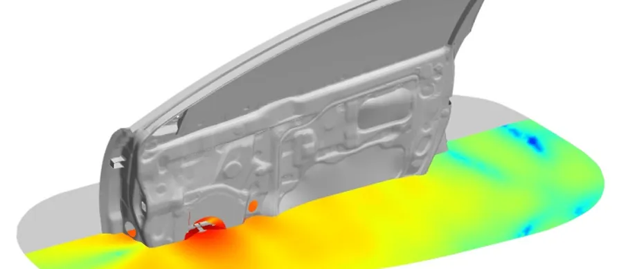
Loudspeaker simulation predicts how a speaker, and the device it sits in, will sound and what will buzz, by coupling the magnetic motor, the moving diaphragm, the enclosure air and port, and the surrounding structure in one model. We build that chain around your existing finite element, CFD and acoustic solvers, so enclosure volume, port geometry, tolerances and fixings are settled before tooling is cut.
The handheld speaker meets its response target on the bench. Then some units from the first build buzz on one bass note when played loud, and the in-car variant rattles at the door trim on another. The tools are cut and the launch date is fixed. Is the fault in the voice coil gap, the port, a loose part or a panel? Nobody can say, because the response plot at normal level looks right.
What is loudspeaker simulation, and why does a lumped model fall short?
The usual starting point is the lumped model of Thiele and Small: an electrical circuit, a mass-spring-damper and an acoustic network, joined by two couplings. A voice coil in the magnet gap gives a force Bl i and a back-EMF Bl v, so u = Re i + Le di/dt + Bl v and M x″ + R x′ + K x = Bl i − Sd Δp, with Sd the diaphragm area and Δp the pressure difference across it. A closed box adds an air spring, Cab = Vb / (ρ c²), that lifts the resonance to fc = fs √(1 + Vas / Vb). A port adds an air mass, and box and port resonate near fb = (c / 2π) √(Sp / (Vb Leff)).
That holds while the diaphragm moves as a rigid piston and the parameters are constants. They are not. IEC 62458:2010 models large-signal behaviour with a lumped-parameter model whose dominant nonlinearities are force factor, stiffness and inductance. Bl falls as the coil leaves the uniform field, the suspension stiffens at large excursion, and inductance depends on coil position and current. Above the piston range the cone breaks up into modes, and port flow separates at high velocity.
A product is harder than a bare driver. The reaction force shakes the device around the enclosure, a cabin or a hand changes what the listener hears, and the faults that bring a speaker back are not in the linear model at all.
- Motor. The voice coil sits in the gap of the magnet structure. Its force is Bl times current and it generates a back-EMF Bl times velocity. Bl and the coil inductance change with position and current, so the motor is nonlinear; electromagnetic finite element analysis gives the curves.
- Diaphragm and suspension. Cone, surround and spider carry the motion. The suspension stiffens at large excursion, and above the piston range the cone breaks up into modes of its own. A structural model of the real parts, not a rigid piston, holds both.
- Enclosure air and port. The trapped air is a spring and the air in the port is a mass; together they resonate at the box tuning. At high velocity the flow separates at the port edges, and a leak adds turbulent noise: acoustic and CFD models carry that.
- Radiation. The front of the diaphragm and the port radiate into the space where the product is heard: a room, a hand, a car door and cabin. The space changes the response as much as the driver does.
- Couplings. Current becomes force through Bl and velocity becomes back-EMF; diaphragm area Sd turns force into pressure and velocity into volume flow. These couplings make the three networks one system. The lumped network is the starting point that three-dimensional models extend.
- Reaction path. The moving mass pushes back on the enclosure, which shakes the panel and fixings it is mounted on. A part with clearance beside that path can strike its neighbour: rattle, outside the transducer and outside any linear model of it.
Where do rub and buzz, port noise and rattle come from?
Klippel's measurement documentation on rub and buzz lists the irregular defects: voice coil rubbing in the gap, buzzing parts, loose particles, hard limiting of the surround and air noise in leaky enclosures. They give impulsive distortion with little energy but a wide-band spectrum, and the page says conventional spectral analysis, as used for THD, is not a sensitive way to detect them because the distortion occurs only within a fraction of a period.
Rubbing is geometry under dynamics. The page notes that at the turning points of the stroke the acceleration is maximal and tilts the voice coil former, so a coil centred at rest can touch the gap wall at one end of the stroke. Whether a unit rubs depends on gap clearance, centring, winding straightness and drive level, and all of them scatter in production.
Rattle lives outside the transducer. The reaction force shakes the enclosure and its mounting, and any part with clearance, such as a battery, a flex cable or a door-panel fixing, strikes its neighbour when a mode of the part or panel sits near a bass tone. Clamping and tolerance make one unit rattle and the next stay quiet. The model needs contact.
Air makes noise too. At high port velocity the flow separates at the port edges and the port chuffs. A leak at the dust cap or in the enclosure makes turbulent noise that Klippel's documentation on air leakage noise describes as audible and perceived as a defect. Chuffing is a CFD question about the port ends; a leak needs sealing data in the model, not geometry alone.
- Coil tilt in the gap. At the turning points of a bass stroke the acceleration is highest and tilts the voice coil former. A coil that is centred at rest can touch the gap wall at one end of the stroke. Clearance, centring and winding scatter decide which units rub.
- Loose part and panel. The reaction force shakes the housing. A part in a pocket strikes the pocket walls when a panel or part mode sits near the bass tone; clamping and tolerance make one unit rattle and the next stay quiet.
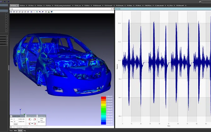
- Short spikes. An impact lasts a fraction of a cycle. In the microphone signal it is a sharp spike riding on the smooth tone, usually at one end of the stroke.
- Spectrum. A smooth tone and its low harmonics are regular distortion. An impact carries little energy but spreads it across a wide band of higher orders, below the level that a figure summing the low orders can show.
- Risk map. A time-domain model with contact is run over displacement and frequency, with sampled tolerances. The map shows where impacts start, so the design moves before tooling and the end-of-line test looks where the risk is.
How is loudspeaker design usually done, and where does it break?
A transducer supplier delivers small-signal Thiele-Small data and a response curve. The enclosure is sized with a lumped model, and listening and a distortion rig judge the prototype. The device team packages electronics, battery and trim around the speaker afterwards, so buzz and rattle appear when assembled units are played loud, after the housing tool is cut.
It breaks at three hand-offs. Small-signal data say nothing about maximum excursion. The speaker and the device are modelled by different teams, so the reaction force never reaches the structure model. And the sound-quality target is set by listening once the design is fixed. The cost is a tooling change, a re-spun housing, or a limiter that gives back the loudness the product was meant to deliver.
How do you simulate a loudspeaker from amplifier to listener?
We build the chain in five stages, and each ends in a check against a measurement you already take.
- Motor and suspension. Electromagnetic analysis in your existing solver gives Bl(x) and Le(x, i); a nonlinear structural model of surround and spider gives K(x). Check: the curves against a large-signal measurement of the kind IEC 62458:2010 describes.
- Diaphragm, enclosure and radiation. A coupled structural-acoustic model in Abaqus, Ansys, Nastran or the acoustic solver Actran carries diaphragm modes, cavity, port and radiation into open air or a car door and cabin. Check: response and impedance at low drive.
- Port and leak flow. CFD in Ansys Fluent or Siemens STAR-CCM+ resolves separation at the port edges and passes the loss to the acoustic model. Check: where port noise starts on the rig.
- Device structure and contact. The reaction force drives housing, panel and fixings in a time-domain finite element or multibody model, in Abaqus, LS-DYNA or your existing solver, with contact for loose parts and for the coil in its gap, as in our flexible multibody and FEA coupling article. Check: an accelerometer sweep on the assembled device at high drive.
- Listener and sound-quality target. IEC 60268-21:2018 specifies physical acoustical measurements for transducers and complete sound systems, automotive systems included, and its scope says it does not assess perceived sound quality. Each simulated metric is therefore tied to a listening test; ITU-R BS.1116 is the ITU method for small impairments in audio systems. Check: metrics rank good and bad units as listeners do.
Then the loop closes: the first prototype's measured sweep updates the parameter curves and damping. The force factor comes from our electromagnetic multiphysics work, not a datasheet.
| Symptom | Likely source | First model to run |
|---|---|---|
| Buzz on one bass note, only when loud | Coil touching the gap, or surround limiting | Large-signal motor model with coil tilt and gap tolerance |
| Chuff or hiss at the port on loud bass | Flow separation at the port edges | CFD of the port in oscillating flow |
| Rattle at one frequency, in some units only | Loose part or panel mode meeting the tone | Housing modes, then contact with sampled tolerances |
| Air noise that follows the cone | Leak at the dust cap or a seam | Leak path with measured seal data |
| Bass below target after the enclosure shrank | Less box volume, or the port tuning moved | Lumped model with the 3D enclosure |
| Peak or dip in the car, not on the bench | Door cavity and panel modes | Vibro-acoustic model of door and cabin |
| Distortion that rises smoothly with level | Bl(x) and K(x) nonlinearity | Large-signal parameters from FEA |
Do not sign off a speaker on its small-signal response
Where does AI help loudspeaker design, and where does it not?
- A surrogate of the motor: Bl(x), Le(x, i) and K(x) as functions of magnet, plate, coil and surround geometry, trained on a planned set of finite element runs, so a motor search becomes affordable. See surrogate models for CFD and FEA.
- Tolerance scatter: gap clearance, centring, clamping and part clearance are sampled through the surrogate and the contact model, giving the share of units at risk of rub or rattle at each drive level, which sets tolerances and the end-of-line limit.
- Calibration: a Bayesian fit of damping and stiffness to impedance, sweep and accelerometer data, returning parameters with their uncertainty. See AI surrogate models you can sign off.
Where it does not help: impacts and flow separation outside its training range. A surrogate built on smooth cases does not know a new port shape, so it carries a stated range and returns anything outside it to the solver. Nor does it replace the listening panel: a model predicts a metric, and whether customers like the sound is a listening result.
From one speaker project to an acoustic design capability you keep
The return comes when your team runs the chain for the next device.
- Physics model. CFD and FEA set up once, as templates: geometry clean-up, mesh, solver settings and post-processing that every later run reuses.
- Validation. Mesh and time-step studies, and comparison with tests or full-scale data, so the model's uncertainty is known before it is trusted.
- Automated runs. Scripted runs over the parameters and operating conditions that matter, on your hardware or in the cloud.
- AI surrogate. A machine-learning model trained on those runs answers in seconds and says how sure it is; low-confidence questions go back to the solver.
- Decision tool. Optimisation, trade-off charts or operating guidance, in a form your engineers and operators use every day.
- Field data. Test, trial and monitoring data flow back to recalibrate the model, so it improves with every project instead of being rebuilt.
- A parameterised transducer-to-device chain in your existing solvers, with the hand-offs between models scripted.
- Automated large-signal runs: each design change is swept over drive level and frequency, and the impact risk map is redrawn.
- A correlation record: impedance, response, large-signal parameters and accelerometer sweeps per variant, with damping and stiffness fitted from them.
- A surrogate with a stated range over motor geometry, port geometry and tolerances, with a gate that returns out-of-range requests to the full model.
- Handover and training, so your engineers extend it. See our training and software development services.
Questions engineers ask about loudspeaker simulation
What is rub and buzz in a loudspeaker?
How do you simulate a loudspeaker?
Are Thiele-Small parameters enough?
Can simulation predict rattle before the device is built?
Which solvers do you use?
If a speaker, or a device with one, is on your desk, send us the transducer drawing and motor geometry, any Thiele-Small or large-signal data, the enclosure and port CAD, the housing and its fixings, and a sweep or recording of a unit that buzzes or rattles. We will reply with how we would build the chain, which hand-off we would check first, which measurement would calibrate it and what the first risk map would let you decide. Start with a conversation, or read about our audio and consumer electronic device design work and the acoustics and vibration section.