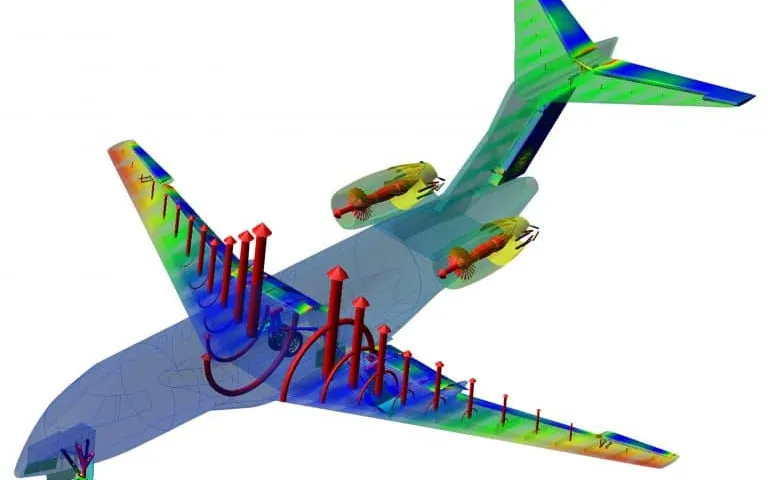
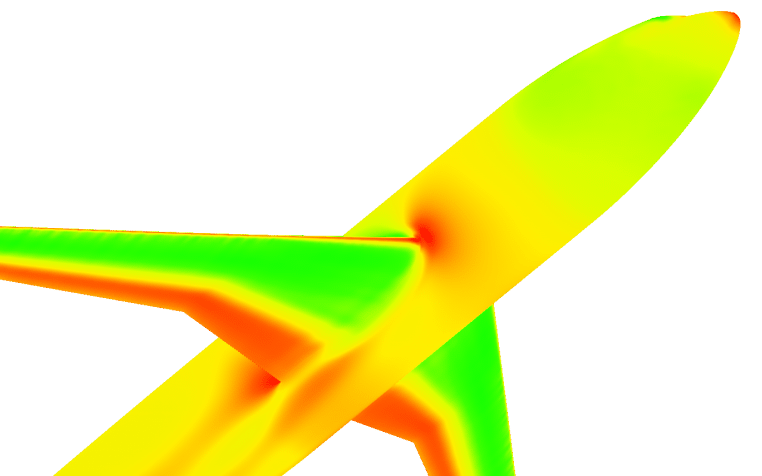
Airframe noise simulation for landing gear and high-lift devices with CFD and FW-H
A gear door or flap change can add a tone that the open-jet entry or flyover test shows only after the hardware is built. Scale-resolving CFD, an FW-H propagation step and a validation record against array data rank the options first.
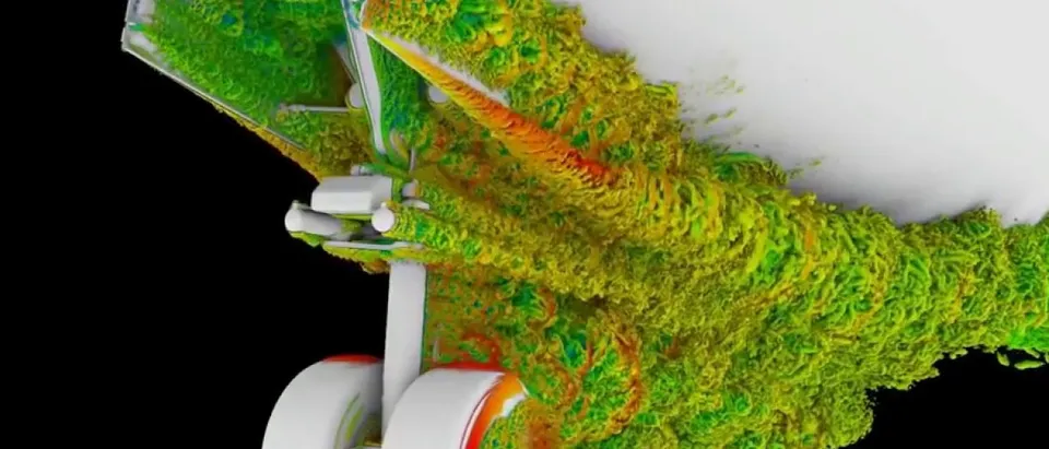
Airframe noise simulation predicts the sound that flow around landing gear, slats and flaps radiates on approach: a scale-resolving CFD calculation resolves the turbulence and a Ffowcs Williams-Hawkings (FW-H) integral carries it to the microphones. We build that chain around your existing solver, so gear fairings, strut shapes and flap settings are ranked on tones and broadband levels before an open-jet entry or flyover test is booked.
The gear-door design freeze is close and the open-jet array slot is booked. If a pin or a door edge sings, you learn it from the array map, with the hardware built. With quieter engines, NASA's overview of the BANC benchmark workshops describes landing gear and high-lift devices as important contributors to the approach noise of subsonic transports. Models do not always transfer: in the 2005 Quiet Technology Demonstrator 2 flight test, two gear noise-reduction concepts chosen in model-scale work showed no reduction in the far-field spectra. Which variant goes to the tunnel?
Why are landing gear and high-lift devices so hard to predict?
The sound is turbulence meeting solid parts. Tones come from vortex shedding off struts and axles, f ≈ St·U/d with St near 0.2 for a circular cylinder at subcritical Reynolds numbers, and from resonances at pins and door edges, which NASA Ames lists among landing gear tones. Broadband noise comes from separated flow, wheel wakes and wakes striking downstream parts. Components interact: in the tandem-cylinder benchmark the rear cylinder is buffeted by the front wake, the sound is mostly tonal, and some computations flipped between two flow states.
And the sound is faint: the BANC overview points to the amplitude and scale gap between flow and acoustic fluctuations, and at Mach 0.2 a sound wave is about five times longer than an eddy of the same frequency (λa/λe ≈ 1/M).
- Strut and axle shedding. Each circular strut or axle sheds vortices in turn, at a frequency that scales with speed over diameter. The pressure on the part pulses at that rate and radiates a narrow tone. Tripping the boundary layer, as the test did, changes the shedding, so the model must match it.
- Wheel wake and shear layers. Flow separates from the wheels and from the strut and trails behind as a turbulent wake. It is the main broadband source, and the wake strikes parts further downstream, which adds noise and ties the components together.
- Bay and door edges. Pins, hinges, the open bay and door leading edges can resonate as the shear layer passes. These are tones, they depend on small geometry, and an under-resolved mesh can invent or hide them.
- Slat cove and flap edge. The shear layer leaving the slat cusp feeds the cove with unsteady flow, and a vortex rolls up at the side edge of a deployed flap. Both radiate on approach, mostly broadband with some narrow peaks.
- FW-H surface. The dashed surface encloses the sources. Flow data on it, solid on the body or permeable off it, is integrated to give the pressure at any observer. The wake leaves through the downstream face, which is where spurious noise appears and where end-cap averaging is applied.
- Ground microphones. The integral treats the air outside the surface as a uniform medium, so each microphone receives the direct path only. Shielding by the wing and refraction by the flow need a further step, and a microphone array adds a beamform map that can be compared with the same map computed from the CFD.
How does airframe noise simulation turn CFD into far-field sound?
CFD cannot carry sound hundreds of metres, so the work is split (Lopes and colleagues). Scale-resolving CFD, compressible or weakly compressible (hybrid RANS/LES, wall-modelled LES, lattice Boltzmann), computes the unsteady flow near the body; an integral method propagates it. The FW-H equation, □²p′ = ∂/∂t[Qδ(f)] − ∂/∂xi[Liδ(f)] + ∂²/∂xi∂xj[TijH(f)], gives a thickness monopole, a loading dipole and a quadrupole volume term. On a solid surface the quadrupole is usually dropped. A permeable surface off the body carries the sources it encloses, but wake crossing it adds spurious noise, which Czech and colleagues reduce by end-cap averaging. Both assume uniform free space, so shielding by the wing and refraction need a boundary element or computational aeroacoustics solver.
Propagation is an error source of its own. On one LAGOON nose-gear solution, two codes with the same formulation on the on-body surface agreed within 0.25 dB from 0.24 to 3 kHz; on the off-body surface three codes spread with a standard deviation of 1.5 dB in the near field and 2.7 dB in the far field (sparse participation). Rotors (eVTOL rotor noise), cabins (wind noise) and engine acoustic liners use the same chain; this article stays with the airframe.
How fine must the mesh and the record be?
A mesh carries the eddies that make sound only up to about f = U/(N·Δ), with Δ the local cell size and N the points per wavelength the scheme needs. In the full-scale lattice-Boltzmann study, the extra-coarse mesh was well resolved to about 1.5 kHz, the coarse mesh to about 2 kHz, and the finest nose-gear mesh matched flight data to 5 to 6 kHz, the highest measured. That nose gear cost 80 thousand CPU hours on the extra-coarse mesh and 4.5 million on the fine one.
A coarse mesh can also invent sound: extra-coarse runs showed tones near 500 Hz and 1 kHz that the flight data lack, and they faded with refinement. The NASA Ames LAGOON study ran six meshes, from 2.2 to 738 million cells: far-field results agreed to 4 kHz and over-predicted above it, yet a 2.4 mm mesh with poor near-field results matched the microphones surprisingly well, so a far-field match can hide a poor near field. The record matters too: levels from 0.3, 0.5 and 0.865 s differed insignificantly in the full-scale case, but a short one limits the FFT frequency resolution.
- Measured spectrum and its band. The reference, from a microphone array or a tunnel. The shaded band is what the facility, the trips and the pass-to-pass variation allow. A prediction inside it is as good as the test can show, and the narrow spike is a tone.
- Coarse mesh and its roll-off. Every mesh carries the eddies that make sound only up to a highest frequency, about speed over points per wavelength times cell size. Above it the computed spectrum drops away. That is the mesh speaking, not the physics.
- Fine mesh, higher band. Refining where the shear layers live moves the roll-off up. Each refinement multiplies the cells and the time steps, so the band is bought, and we state which one a run carries.
- Spurious tone. An under-resolved shear layer or cavity can ring at a frequency the test does not show. It fades as the mesh is refined, so no tone is trusted from one mesh.
- Propagation spread. The same flow data, passed through another surface or solver, shifts the far-field level. It adds to the mesh error, so we check propagation on identical input.
- Cells per wavelength. At one frequency the sound wave is about 1/M times longer than the eddy that makes it. The same cells hold the sound easily and the eddy poorly; the eddy is smeared first, and that sets the roll-off above.
How do array and wind-tunnel data check the prediction?
The BANC overview reports spectra from a closed-wall aerodynamic tunnel differing by more than 3 dB from open-jet data because of reverberation, and tandem-cylinder side plates adding 1 to 2 dB to the overall level while spanwise periodic boundaries kept coherence higher than the tunnel's. Narrowband peaks on a slat proved highly sensitive to boundary-layer trips, so broadband levels were the sturdier comparison.
For arrays, put the CFD data through the same beamforming. Czech and colleagues built synthetic records at the flight-test microphone positions, against a 614-microphone array whose pass-to-pass scatter was about 2.5 dB above 200 Hz. The coarse mesh was within about 2 dB to 2 kHz for the main gear in landing configuration; at the aft emission angle the nose gear was under-predicted by 2 to 3 dB, which the authors conjecture is residual engine noise rather than the mesh. Beamform maps can also steer meshing: for one high-fidelity nose gear, array data pointed to the shock strut and torque arms, and refining there matched most of the spectrum closely.
A gear ranking is not an aircraft noise level
What does noise certification ask of a prediction?
ICAO's noise standards sit in Annex 16 Volume I, with three reference measurement points; ICAO says certification should ensure that the latest noise reduction technology is built into designs and demonstrated by procedures relevant to daily operations. Its page records Chapter 14, 7 EPNdB cumulative below Chapter 4, for new types from 31 December 2017 (2020 below 55 tonnes), and a Chapter 16 adopted on 27 March 2026, six decibels stricter for large types and two for smaller ones, for new type designs from 2029.
In the United States, 14 CFR 36.101 requires transport category large airplane noise to be measured and evaluated under Appendix A or an approved equivalent procedure; the appendix notes that the FAA permits approved equivalent procedures, for example for minor changes to a type design. The metric, EPNL = PNLTM + D, is built from 24 one-third-octave bands from 50 to 10,000 Hz at half-second steps, with a correction for the maximum tone: a strong gear tone costs certified level. The bands reach 10 kHz, beyond the 5 to 6 kHz at which the finest mesh above met flight data. We found no wording that makes a CFD prediction a means of compliance; simulation plans the test, chooses what to fly and explains the result.
| Question | Method | What it can miss | Use it when |
|---|---|---|---|
| Which gear or fairing is quietest? | Isolated gear, scale-resolving CFD, on-body FW-H | Wing downwash, shielding | Screening many variants |
| Is there a tone, and where? | Hybrid RANS/LES or wall-modelled LES, two meshes, trips as tested | Tones that exist only on a coarse mesh | Pins, door edges, struts |
| What reaches the ground? | Installed gear, flap and wing, permeable FW-H with end caps | Refraction, shielding | Flyover or sideline estimate |
| Where is the source? | Beamforming of CFD data, processed like the test | Low-frequency resolution | Choosing where to refine or fair |
| Do slat or flap edges matter? | Quasi-2D, then 3D hybrid RANS/LES, span checked | Spanwise cut-off, brackets | High-lift setting |
| Which of hundreds of variants to run? | Surrogate calibrated on validated runs | Geometry outside its range, tones | Design-space screening |
Where does AI help airframe noise screening, and where does it not?
- Surrogate screening. Trained on validated CFD-to-FW-H runs over fairing size, strut shape, flap setting and speed, a surrogate returns one-third-octave spectra at observers for many variants, and finalists go back to the full chain. NASA's overview expects BANC data to serve reduced-order models. See surrogate models for CFD and FEA and reduced-order modelling.
- Calibration. Empirical component models are fitted to validated runs and return parameters with a range.
- Gates. A mesh comparison flags tones that move or vanish on refinement; array spectra that break the speed trend are held back. See AI surrogate models you can sign off and uncertainty quantification.
It does not help outside its training: a new gear architecture is a new problem, and a tone that switches on at a resonance is not smooth, so we classify it and send anything near a resonance to the full chain. The physics chain stays the evidence; the surrogate chooses the runs.
From one gear study to an airframe noise workflow you keep
The return comes when your acousticians put the next fairing, door or flap through the same chain, against the same validation record.
- Physics model. CFD and FEA set up once, as templates: geometry clean-up, mesh, solver settings and post-processing that every later run reuses.
- Validation. Mesh and time-step studies, and comparison with tests or full-scale data, so the model's uncertainty is known before it is trusted.
- Automated runs. Scripted runs over the parameters and operating conditions that matter, on your hardware or in the cloud.
- AI surrogate. A machine-learning model trained on those runs answers in seconds and says how sure it is; low-confidence questions go back to the solver.
- Decision tool. Optimisation, trade-off charts or operating guidance, in a form your engineers and operators use every day.
- Field data. Test, trial and monitoring data flow back to recalibrate the model, so it improves with every project instead of being rebuilt.
- A geometry ladder in your existing solver: levels of detail (hoses, bolts, hinges in or out), tripping as tested, speed and flap setting as inputs.
- Mesh and record rules with the highest resolved frequency stamped on every run.
- Automated CFD-to-FW-H runs: solid and permeable surfaces, end caps, observers at your array positions, one report.
- A post-processor for narrowband and one-third-octave spectra, tone flags and beamform maps processed like your tests.
- A validation record: facility, trips, array processing, scatter, date.
- A surrogate with a stated range and a gate to the full chain.
- Handover and training, so your team runs and extends it. See our training and software development services.
Questions engineers ask about airframe noise simulation
Can CFD predict landing gear noise?
Should the FW-H surface be solid or permeable?
Why does my simulation show a tone the test does not?
Can simulation replace the noise certification test?
Is a wind-tunnel test enough without simulation?
If a gear, door or flap change is waiting on a noise answer, send us the geometry and its level of detail, the speed and configuration, observer or array positions, any test spectra, and the band and metric the decision uses. We reply with how we would build the chain, the highest frequency each mesh would carry, what the validation record should hold and what a surrogate could cover. Start with a conversation, or read the aerodynamic noise simulation page and the aeroacoustics practice.