Resistance spot welding simulation for weld lobes, nugget size and joint strength
A new grade or stack-up reaches the line, and the weld schedule, the nugget diameter and the failure mode for the crash model are all open. Coupled electrical-thermal-mechanical simulation predicts nugget growth, expulsion and the weld lobe before the first coupon.
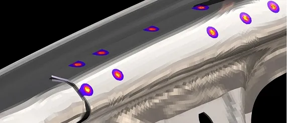
Resistance spot welding simulation solves the coupled electrical, thermal and mechanical problem in the electrode and sheet stack to predict nugget growth, expulsion and final size, so a weld schedule can be set before a coupon is welded. We build it around your existing solver as a workflow your team runs, with a weld-lobe surrogate and a hand-off to your crash and fatigue models.
A reinforcement in a new high-strength grade joins a stack-up your line has welded in mild steel for years. At the old current the nuggets are small; a few kiloamperes higher, the welds expel. Process engineering needs a schedule before the launch build, the crash team needs a nugget diameter and a failure mode, and the next coupon slot is weeks away. The Nippon Steel & Sumitomo Metal Technical Report No. 119 notes that the number of spot-welded locations per body structure has increased.
What does resistance spot welding simulation have to predict?
Four things for each stack-up: how the nugget grows with current, time and force; where the weld window ends, at the current that gives the required nugget size and the current that expels molten metal; how the window moves with electrode wear and shunting; and what the joint is once welded, meaning nugget diameter, heat-affected zone, strength and failure mode.
The window is drawn as a weld lobe. The Nippon Steel report charts nugget diameter against current and against electrode force or weld time. ISO 18278-2:2016 gives test procedures for the acceptable current range and the electrode life, and AWS D8.9M:2022 presents test methods for current range, electrode endurance and weld properties of automotive sheet steels. A lobe test gives the window of the coupon welded. A model gives the window of the stack-up on your drawing.
Why is a spot weld harder to model than it looks?
A spot weld couples three fields that feed back on each other. Current heats the stack by Joule heating, Q = ∫ I2(t) R(t) dt, where R is the bulk resistance of the sheets, which rises with temperature, plus the contact resistances at the electrode faces and between the sheets. Those depend on contact pressure and area, on films and coatings, and on temperature, and pressure and area come from the mechanical solution.
That loop is why the Nippon Steel approach alternates a coupled electrical-thermal analysis with a coupled thermal-mechanical one at small intervals, with phase change included. The authors single out contact resistance: it fades once current flows and looks unimportant, yet ignoring the interface heating leaves too little heat at the start of the weld to predict the nugget.
Materials add physics. On coated steel the coating melts and is pushed out of the contact, widening the current path until it evaporates, and the nugget forms more slowly. High-strength steel has a higher resistivity than mild steel from room temperature to 1,000 °C, so in a mixed stack it melts more. Aluminium conducts so well that it needs far more current, its oxide film adds contact resistance, and electrode life is short: the TWI literature survey of 1979 named that among the major factors limiting spot welding of aluminium alloy sheet.
- Cooled copper electrodes. The electrodes press the sheets together and carry the current in. Water cooling draws heat out of the outer surfaces, so the hottest region is the interface between the sheets. As the tip face wears and broadens, the same current spreads over a larger area and heats the interface less.
- Current path. Current runs from tip to tip and has to squeeze through the contact between the sheets. The path changes as the contact area grows and as the nugget forms, so the electrical problem cannot be solved once and left alone.
- Contact resistance. At the interface the surfaces touch only at their asperities, and current constricts through those points. Contact pressure, surface film, coating and temperature set this resistance, and it dominates the heating at the start of the weld. A model that ignores it under-heats the start of the weld.
- Nugget. Molten metal forms at the interface and grows through both sheets while heat is generated faster than it conducts away. Its diameter is the size that acceptance criteria and crash joint models both ask for.
- Heat-affected zone and corona bond. Around the nugget the steel is heated without melting, and its microstructure changes. In high-strength steels this zone can soften or harden and decides where a joint fails. The ring where the sheets stay pressed together outside the nugget, the corona bond, holds the molten metal in.
- Expulsion. When the electrode force and the corona bond can no longer contain the molten metal, it is thrown out between the sheets. Expulsion is a threshold event and marks the upper edge of the weld lobe.
- Joule heat balance. The heat generated in the stack is the integral of current squared times resistance over time, and the resistance itself changes through the weld. The heat generated where resistance is highest, less the heat conducted away into electrodes and sheets, is what grows the nugget.
How are spot-weld schedules usually set, and where does that break?
By lobe testing and experience: weld coupons across a current range, section them, choose a schedule mid-window and release it with a tip-dressing rule. AWS D8.1M:2021 states acceptance for resistance spot welds in steels as visual and measurable criteria. That suits the coupon. Four things break it on a structure.
- Shunting. In the Nippon Steel door-opening model, with existing welds 25 mm away, only 60 to 80% of the 7.0 kA input reached the weld, and the nugget ended considerably smaller than on a single-spot coupon.
- Gaps. A coupon with spacers does not reproduce the gaps of a formed part. In the same report one gap arrangement sped nugget growth and another slowed it.
- High-strength steel. The open-access Metals study of complex-phase steel by Morales-Sánchez, Collazo and Doval-Gandoy notes that these steels tend to fail at the interface, so a large button diameter does not always result in button failure.
- Electrode wear. The tip face grows and the same current heats the weld less, so the new-tip lobe is not the end-of-dressing lobe. That is why ISO 18278-2 pairs the current range with the electrode life.
| Question | Physics model | What it hands over | Decision it supports |
|---|---|---|---|
| Schedule for a new stack-up | Axisymmetric electrical-thermal-mechanical model with contact resistance | Nugget growth history, lobe edges | Which trials to weld |
| Shunting and pitch in an assembly | 3D flange model with neighbouring welds, gaps and stiffness | Current reaching the weld, nugget size | Pitch, weld order, gap tolerance |
| Expulsion margin | Contact force around the nugget, calibrated criterion | Upper lobe edge | Distance of the schedule from expulsion |
| Electrode wear and dressing | The same model with a worn tip face | Lobe shift with tip condition | Dressing interval, current stepping |
| Joint strength in crash or service | Nugget and heat-affected-zone properties, fracture criterion | Strength and failure mode by load case | Spot count, diameter and pitch |
| Many stack-ups | Planned runs of the physics model | Lobe surrogate with a gate | Which stack-ups need a full run or a test |
How do you build a spot-weld model you can rely on?
We set the coupled model up in your existing solver, such as LS-DYNA, Ansys or Abaqus, implementing the contact-resistance law and phase change where the solver lacks them. Our welding simulation hub and resistance spot welding page give the wider context.
Done properly, three records come with it. Verification: mesh refinement in the contact zone, time-step convergence and an energy balance between electrical power and stored and conducted heat. Validation: nugget growth from interrupted welds, cross-sections, the resistance signal and the lobe edges, with tolerances set before the run. The Nippon Steel report compares nugget growth, cross-sections and lobes for mild, 590 MPa and 980 MPa dual-phase steel and reports favourable agreement. Uncertainty: contact-resistance parameters, surface condition, material data, alignment and gap, varied so the lobe comes with a band.
The report predicts expulsion when the contact force at the ring around the nugget falls to (1 − k) times the electrode force; k, near 0.9 in the authors' experiments, absorbs electrode misalignment and machine effects. Your machine gives your own k, so we fit it to a few of your welds and test it on others.
- Undersized nugget. Too little current or too short a time leaves a nugget smaller than the size your acceptance criterion asks for. The weld exists but sits outside the window.
- Lower edge: minimum nugget size. The contour where the nugget just reaches the required diameter. In a published lobe prediction from Nippon Steel the lower edge is the contour of a nugget diameter of 4√t, with t the sheet thickness in millimetres.
- Weld window. The schedules between the two edges. Its width is the process margin: a schedule near the middle tolerates variation in force, fit-up, coating and tip condition, and one near an edge does not. The dot marks a chosen schedule.
- Upper edge: expulsion. Beyond this edge the molten metal escapes. It is a threshold, so the physics model needs an expulsion criterion calibrated on your machine, and a surrogate needs a gate here.
- Drift from wear and shunting. As electrode tips wear, and as neighbouring welds shunt current away, the same set current heats the weld less, so the window moves towards higher current. A schedule that sat in the middle of a new-tip lobe can sit at its lower edge later.
- What the weld model hands on. Nugget size, the heat-affected zone and the state of the nugget metal go to the crash joint model, which needs them to set strength and failure mode. The fatigue model needs the nugget edge geometry from the weld model and the load on each spot, with its peel component, from the structural model.
A predicted lobe is not a qualified schedule
What must a spot-weld model hand to crash and fatigue models?
The Nippon Steel report states the stakes: if the nugget diameter or weld pitch differs from the drawing, the weld may fracture under collision deformation. Our article on crash model credibility covers how the connection model is built and checked. The weld model supplies its inputs.
- Nugget diameter and position, with scatter, for the stack-up and weld order as built.
- Heat-affected zone extent and hardness. In dual-phase steels, the Metals study explains, the zone softens through tempering of martensite, more as strength rises.
- Nugget metal properties. In a dissimilar stack the nugget mixes both sheets. The Nippon Steel team took the mixing ratio from the weld simulation to build the flow curve and fracture limit, and for two of five stack-ups the L-shaped joint strength error fell below 10%, against 10% or more with a mix by sheet thickness.
- Failure mode and strength per load case. In those tests every tensile-shear joint failed at the nugget interface and every L-shaped joint unplugged, so a joint model calibrated on one load case does not carry to the other.
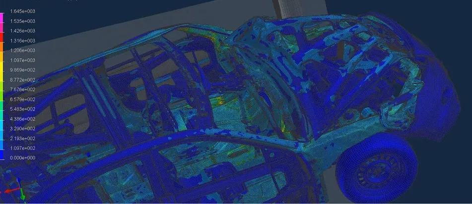
Fatigue needs different data. TWI reports that in shear a spot weld may reach 106 cycles at up to 20 or 25% of its static failure load, but in peel at only about 5%. Fatigue data are normally given as applied loads, so the model needs the load on each spot, with its peel component, from the structural analysis, plus the nugget edge geometry from the weld model. TWI adds that limited nugget porosity does not affect fatigue, that a larger weld gives only a small benefit, and that reducing the peel load on a spot improves performance. Our durability and fatigue work picks up from there.
Where does AI help spot-weld simulation, and where does it not?
- A weld-lobe surrogate. Planned runs of the physics model over thickness, grade, coating, force, schedule and tip condition train a surrogate that returns the lobe edges for a new stack-up without a full run. Its range is stated, and cases near the expulsion edge go to the full model.
- Calibration. Fitting contact-resistance and expulsion parameters to your cross-sections and resistance signals is an inverse problem, solved with uncertainty estimates and kept reproducible.
It does not replace the physics. A surrogate cannot predict a coating, grade or geometry outside its range, inherits the errors of the model it learned from, and never decides whether a nugget is acceptable. See AI surrogate models you can sign off for how we bound them.
From one weld study to a spot-weld capability you keep
The return comes when your engineers can run the next stack-up, grade or coating through the same chain without rebuilding the model or the checks.
- Physics model. CFD and FEA set up once, as templates: geometry clean-up, mesh, solver settings and post-processing that every later run reuses.
- Validation. Mesh and time-step studies, and comparison with tests or full-scale data, so the model's uncertainty is known before it is trusted.
- Automated runs. Scripted runs over the parameters and operating conditions that matter, on your hardware or in the cloud.
- AI surrogate. A machine-learning model trained on those runs answers in seconds and says how sure it is; low-confidence questions go back to the solver.
- Decision tool. Optimisation, trade-off charts or operating guidance, in a form your engineers and operators use every day.
- Field data. Test, trial and monitoring data flow back to recalibrate the model, so it improves with every project instead of being rebuilt.
- A stack-up and schedule file holding grades, thicknesses, coatings, gap, electrode, force, current and time, so a new joint is a line of input.
- An electrical-thermal-mechanical template in your existing solver, with the contact-resistance and coating laws and its checks built in.
- A validation record against your cross-sections, resistance signals and lobe tests, with tolerances set before the run.
- A lobe surrogate with a stated range and a gate at the expulsion edge.
- A hand-off writer that exports nugget size, heat-affected zone, nugget properties and failure data in the format your crash and fatigue models read.
- Handover and training, so your team extends it itself. See our training and software development services.
Questions engineers ask about resistance spot welding simulation
What is a weld lobe?
Can simulation replace lobe testing or weld qualification?
Why is aluminium harder to spot weld and to simulate?
Does a larger nugget always give a stronger joint?
If a weld schedule or a joint model is waiting on a nugget, send us one problem stack-up: grades, thicknesses and coatings, electrode and dressing rule, current schedule, and any lobe tests, cross-sections or failure data, plus the crash or fatigue criterion the weld feeds. We reply with how we would set up the model, what we would calibrate first and on which welds, and what the hand-off should contain. Start with a conversation.