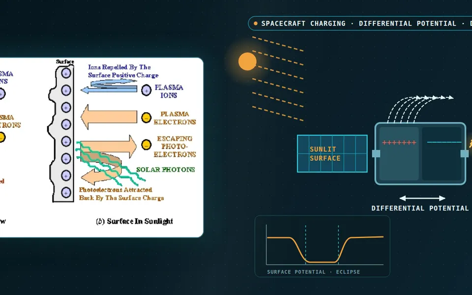
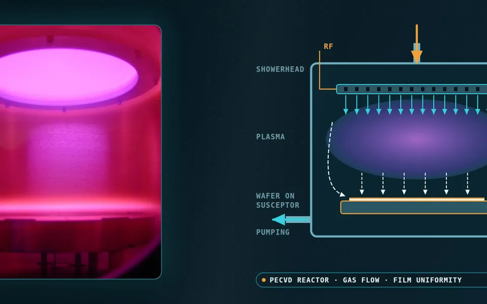
Atmospheric plasma treatment simulation for surface cleaning, bonding and coating
The head cleaned last month's coupons well; this month the water-drop test wanders and a new part peels at the corner. Simulating the discharge, the air-mixing plume, the surface chemistry and the heat load shows which species reach the part and where the process window lies.
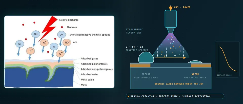
Atmospheric plasma treatment cleans and activates a surface by delivering reactive species to it, mainly atomic oxygen, hydroxyl, ozone and nitrogen oxides, in the seconds a jet or barrier-discharge head spends over each patch of the part. Simulation shows which species arrive and how evenly as gap, flow, power and speed change, so the window for bonding, coating or painting comes from physics and is confirmed on your parts. We build it around your solver, with a validation record and a surrogate.
The line is qualified, yet the water-drop test now wanders, a new part peels at a corner, and no one can say whether the gap, the air in the hall or the head is to blame. The next part's window waits on a coupon lot at line cost. Wetting alone does not settle it: Mui and colleagues took the water contact angle on AA1100 aluminium from 87° to 8° with a plasma jet and 13° with a dielectric barrier discharge (DBD) at about equal surface free energy, yet in the ASTM D3359 tape test jet samples lost no paint (class 5B) and DBD samples ran from 1B to 4B.
How does atmospheric plasma treatment clean and activate a surface?
At 1 bar the mean free path is so short that plasma species arrive with very low kinetic energy; Mui and colleagues note that sputtering is therefore not possible at atmospheric pressure and etching in air is very mild. What reaches the part is a flux of neutral radicals and long-lived molecules, carried by flow and diffusion, that oxidise adsorbed organic films and leave polar groups.
At the surface the flux is two resistances in series, 1/keff = δ/D + 4/(γ⟨v⟩): boundary-layer thickness δ, diffusivity D, reaction probability γ and mean thermal speed ⟨v⟩ (small γ). A high-γ species is limited by the flow, a low-γ one by the surface chemistry.
The outcome you measure is a proxy. ISO 19403-2:2024 (Paints and varnishes, Wettability, Part 2) specifies, per its catalogue scope, a contact-angle method for surface free energy and notes that morphological and chemical homogeneity influence the result; Mozetič adds that water contact angle depends on impurities and roughness. We calibrate your outcome against the species dose on your coupons.
Why are plasma jets and barrier discharges hard to simulate?
One process spans many scales. Schmidt-Bleker and colleagues, studying an argon jet with a shielding-gas device, report guided streamers at several kilometres per second and downstream chemistry over several seconds. Their flow is turbulent (Re ≈ 3000, 3 slm of argon, 1.6 mm nozzle) and the surrounding gas folds in. That gas is the reagent: in their sensitivity study more O2 speeds the conversion of O to ozone, and feed-gas humidity removes O through OH and HO2. Our chemical reactor article treats the same mixing-against-reaction-time question.
- Streamer head in the feed-gas channel. A guided streamer runs down the noble-gas channel in nanoseconds, following the flow, and each pulse makes primary species at its head: excited atoms and molecules, atomic oxygen and nitrogen. A resolved discharge model computes one such event on a converged grid; the production rates it returns are what the slower models need, not the whole plume.
- Air folds in at the plume edge. Turbulent eddies draw ambient nitrogen, oxygen and water vapour into the jet. This is the reagent supply: it converts and destroys the primary species and shifts with the gap, the flow, a shielding-gas curtain and room humidity. The instantaneous air density the streamer meets is below the Reynolds-averaged mean, so the mixing parameter is calibrated, not assumed.
- Short-lived species fade, long-lived ones arrive. Atomic oxygen and hydroxyl are consumed in the mixing zone: oxygen forms ozone, and OH and HO2 take O away. What is left at the surface therefore depends on the gap and the flow speed. Ozone and nitrogen dioxide persist. A downstream reading sees only the survivors, which is why far-field composition differs from the plume.
- A boundary layer, then a reaction probability. In the thin layer beside the part, species cross by diffusion and meet the surface, where a reaction probability decides what sticks. The two resistances act in series: a fast surface reaction is limited by the flow that sets the layer, a slow one by the surface chemistry. The wall jet that forms on the part sets the thickness.
- What the species meet on the surface. The stack on the part is the contamination to be oxidised: adsorbed water and an organic film over the oxide. Where it is removed, the exposed oxide carries polar groups and the drop spreads, a falling contact angle. Roughness and impurities also move the angle, so it is calibrated against adhesion, not read as the property itself.
- The chain the model carries. One resolved discharge event gives production rates; a turbulent flow and reduced-chemistry model carries them through the mixing zone; a boundary layer model returns the flux to the part. Each stage is validated on its own measurement, because the reduced stages are not self-consistent and need close correlation to data.
A barrier discharge splits it differently. Brandenburg describes a gap typically 0.1 to 10 mm behind a dielectric barrier. Each breakdown charges the barrier surface, the charge opposes the applied field and the discharge extinguishes, keeping the plasma non-thermal. In air at 1 bar and a 1 mm gap the filaments last about 10 to 100 ns and transfer 0.1 to 10 nC, too briefly for significant gas heating. Each spreads along the dielectric far beyond its channel, so the part sees a statistical field of footprints.
How do fluid models treat streamers and filaments, and where do they fail?
A fluid model solves drift-diffusion for electrons and ions with Poisson's equation, using transport data from cross sections. Bagheri and colleagues compared six such codes on positive streamers in dry air with identical models and transport coefficients: at each group's standard grid, streamer velocity and maximum field varied considerably; close convergence needed about a micrometre, and run times ran from minutes to days. At very low background ionisation the continuum assumption fails.
Chemistry adds a second uncertainty. Turner reports predicted species densities uncertain by a factor of ten or more in some cases; in a helium–oxygen set of almost four hundred reactions, about fifty rate constants matter and as few as ten cause most of the uncertainty. That says where calibration pays.
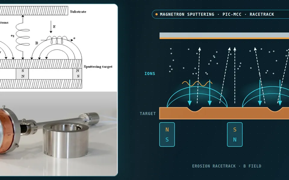
So we do not run one resolved model for everything. Schmidt-Bleker and colleagues link a fast electron-impact model of the streamer head to a slower neutral plug-flow model through a metastable-argon source; it matched measured ozone, NO2 and N2O5 well and over-predicted N2O by more than a factor of two. Other groups reuse the production rates of one detailed discharge event over hundreds of pulses. We build that chain for your head: a converged resolved event (fluid or PIC-MCC; see our plasma-based devices work), production rates into a turbulent-flow, reduced-chemistry model of plume and part, and measurements to close the loop, because the authors state the approach is not self-consistent.
Mixing needs the same care. In that study the streamer sees less ambient air than the Reynolds-averaged mean, and the diffusion coefficient they use is five times the molecular value but about half the Reynolds-averaged one. We calibrate such a parameter, or resolve the plume on one case, and carry it into the sweep.
What sets treatment speed, uniformity and part heating?
Speed is dwell time. A head with footprint d moving at speed v leaves each patch under it for about d/v; energy per area is power times that time over the footprint area. Mui and colleagues matched energy per area (44 and 108 J/cm²) between jet and DBD, taking 40 s with the jet and 6.5 to 44 minutes with the DBD, and adhesion still differed; they point to plasma composition. Dose is bookkeeping; the species mix per unit dose is the variable.
Uniformity is footprint overlap and geometry. Flow stagnates on a flat part, accelerates over an edge and separates in a recess, each changing δ and so the flux, so a coupon result does not transfer to the next geometry. We run the species model on the real part with the head moving and return flux and dwell maps.
Heat is the other edge. Turner notes that the jets he models are power-limited to prevent significant gas heating, yet the part still takes an energy flux over the footprint. We solve the part as a conjugate heat-transfer problem with the footprint moving at line speed (see our thermal analysis), so a film and a casting each get a temperature history; your material limit sets the edge of the window.
- Filaments in the gap. In a barrier discharge the breakdown channels are many thin filaments that flash at random places and spread along the dielectric surface far beyond their own width. The part receives a statistical field of footprints, so uniformity is a question of how many overlap in the time the part spends under the cell.
- The barrier limits the charge. Each breakdown leaves charge on the barrier surface; that charge opposes the applied field and the filament extinguishes. The limit keeps the plasma non-thermal, and the charge left behind is a memory that shapes where and when the next filament forms. Without the barrier the discharge would constrict to a spark or arc.
- Four time scales, four models. Filament and streamer physics runs in nanoseconds and is handled by a fluid or PIC-MCC model of one event. Gas transit and plume chemistry run in milliseconds in a flow and reduced-chemistry model. Dwell, heating and surface activation take seconds. Ageing takes days and is fitted to data. Each rung passes rates to the next.
- Dwell and dose. A footprint of width d moving at speed v dwells for about d over v, and the energy per unit area is power times dwell over footprint area. Matching this dose between a jet and a barrier discharge did not match adhesion in the study cited in the text, so dose is bookkeeping; the species delivered per unit dose is what the model follows.
- Contact angle falls, then levels off. With rising dose the water contact angle falls and flattens, so treatments that differ in adhesion can look alike on the plateau. The window opens where the surface is cleaned and wetted and closes on the right at the heat the part can take. A surrogate maps it, with a gate to the full model at its edges.
- The window has an edge in time. After treatment the angle drifts back up, close to logarithmically in air in the studies reviewed, and faster when the part is warmer. The activation at the moment of coating is therefore set by the delay and the storage temperature, which are inputs to the model and are calibrated on your material.
Which plasma-treatment question needs which model?
| Question | Model | Reports | Limit to state |
|---|---|---|---|
| Which species leave the head? | Fluid or PIC-MCC event | Production per pulse | Grid; reaction set |
| What does the part see at this gap and flow? | Turbulent flow, air entrainment, chemistry | O, OH, O3, NO2 flux maps | Mixing closure, humidity |
| Is a curved part treated evenly? | Same model, moving head | Flux and dwell maps | Footprint calibrated |
| How hot does the part get? | Conjugate heat transfer, moving footprint | Temperature history | Footprint heat flux measured |
| Which gap, flow, power and speed pass? | Surrogate on designed runs | Window map and gate | Valid inside its sampled range |
A predicted species flux is not a qualified process
How credible is a plasma treatment simulation, and what validates it?
Verification means grid, time-step and turbulence-model sensitivity. Validation must happen where the part is: Schmidt-Bleker and colleagues find the far-field composition measured by FTIR very different from the species expected in the plume, so a downstream ozone reading is not the flux to the surface. We validate effluent species where measurable, contact-angle maps over a scanned coupon, and the adhesion test on the real stack, and sample the dominant rate constants, humidity and mixing parameter.
Time belongs in the model. Mozetič's review of plasma-activated polyethylene finds hydrophobic recovery thermodynamically driven, present even in vacuum, faster when warmer and almost logarithmic in air over the up to one month most authors studied. The angle right after treatment is not the state at coating: delay and storage temperature are process inputs.
Where does AI help plasma process design, and where does it not?
- Surrogates over the window. Trained on designed runs of the coupled chain over gap, flow, power and speed, a surrogate returns species flux, dose and part temperature in seconds within a stated range, with a gate outside it. The jet study's reduced chemistry runs in 3.7 s.
- Calibration. An inverse fit of rate constants, mixing parameter and surface reaction probabilities to your measurements returns ranges.
- The surface response. A small model links delivered dose to contact angle, adhesion class and ageing, trained on your coupons, range stated.
It does not repair a wrong reaction set, extrapolate beyond the gas, material or head the data covered, or replace the coupon lot. See our hybrid physics-AI, surrogate modelling and uncertainty quantification pages and our articles on surrogate models and validating them.
From one process study to a plasma-treatment workflow you keep
The return comes when your engineers can put the next head, part or line speed through the same chain.
- Physics model. CFD and FEA set up once, as templates: geometry clean-up, mesh, solver settings and post-processing that every later run reuses.
- Validation. Mesh and time-step studies, and comparison with tests or full-scale data, so the model's uncertainty is known before it is trusted.
- Automated runs. Scripted runs over the parameters and operating conditions that matter, on your hardware or in the cloud.
- AI surrogate. A machine-learning model trained on those runs answers in seconds and says how sure it is; low-confidence questions go back to the solver.
- Decision tool. Optimisation, trade-off charts or operating guidance, in a form your engineers and operators use every day.
- Field data. Test, trial and monitoring data flow back to recalibrate the model, so it improves with every project instead of being rebuilt.
- A parametric head-and-part model in your existing solver: head, gap, gas, flow, power, speed and geometry as parameters, one template recording mixing, mesh and time-step choices.
- A chemistry library with sources, ranges and the dominant rate constants flagged.
- A validation record against effluent species, a scanned coupon and your adhesion test, with tolerances set first.
- A surrogate with a stated range and a gate to the full model.
- Handover and training, so your team runs and extends it. See our training and software development services.
Questions engineers ask about atmospheric plasma treatment simulation
Can simulation predict the contact angle?
Do I need to simulate the discharge, or only the gas flow?
How do jets and barrier discharges differ for simulation?
Can the simulation show whether my ozone and nitrogen oxide emissions are safe?
Which solver do you need?
If a new part, a faster line or a changed head waits on a process window, send us the head drawing with its operating range, the part and material, the gap and speed range, your outcome test and time to coating, and any species or temperature data. We reply with the model chain we would set up, the validation we would run and what a surrogate could cover. Start with a conversation, or see our plasma cleaning page.