Wind turbine CFD for blade loads, wake losses and wind farm layout
A wake-loss figure sits in the yield model and the layout is about to freeze, but the model was tuned for flat ground and neutral air. Blade-resolved CFD, actuator models and calibrated engineering models, each used where it is valid, put rotor, wake and layout on one validated chain.
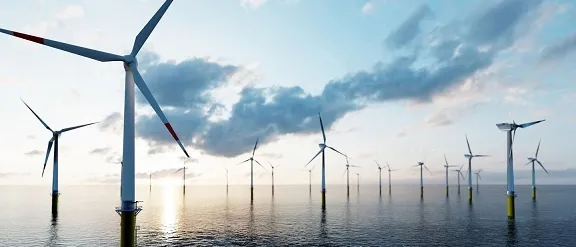
Wind turbine CFD predicts the flow through a rotor and the wake it leaves, so a blade design, a turbine spacing or a yaw schedule can be compared before a prototype blade is built or a layout is frozen. No single model answers every question: blade-resolved CFD serves the rotor, actuator models serve the wake and fast engineering models the layout, each only as far as it has been checked. We set that chain up around your existing solver, with its validation record.
The layout freeze is close. A wake-loss figure sits in the yield model, calibrated on flat ground and neutral air, not on the ridge, the stable nights or the closer row now proposed. The AWAKEN page of the U.S. National Laboratory of the Rockies says industry models used to predict turbine-to-turbine wake losses have uncertainty levels of 20%–50%, and that the campaign exists to cut them. At blade level, loads, structural sizing and the test slot depend on aerodynamics whose weak regimes you need to know early.
What does wind turbine CFD have to resolve, from blade to wind farm?
A rotor extracts power P = ½ρAU3CP and pushes on the air with thrust T = ½ρAU2CT, and momentum theory caps CP at the Betz limit, 16/27 ≈ 0.593. The review by Porté-Agel, Bastankhah and Shamsoddin (2020) describes what follows: a near wake two to four rotor diameters long, with helical tip and root vortices shed at the blade-passing frequency, then a far wake whose deficit is close to a Gaussian, ΔU/U∞ = [1 − √(1 − CT/(8(σ/d)2))] exp(−r2/(2σ2)), r the distance from the axis, with width σ/d = kx/d + ε growing roughly linearly.
The growth rate k is not a constant: the review quotes k ≈ 0.38I + 0.004 for inflow turbulence intensity I between 0.06 and 0.15. Eddies larger than about two rotor diameters carry the whole wake sideways, and turbines three to ten diameters apart usually sit inside it, so inflow turbulence and meandering matter more to a farm than rotor detail.
- Inflow with large eddies. The atmospheric boundary layer is turbulent over a huge range of scales. Eddies much larger than the rotor do not mix the wake, they carry it sideways. The turbulence imposed at the inlet therefore sets how fast the wake recovers and how far it wanders, so the inflow is a model input, not a detail.
- Near wake and tip vortices. For the first two to four rotor diameters the flow still carries the blades: a helix of tip vortices, a hub vortex and strong shear. A blade-resolved or actuator-line model has to keep them alive without numerical smearing; an engineering wake model usually starts beyond them.
- Far-wake deficit. Further downstream the time-averaged deficit is close to a Gaussian, the same shape at every station: shallower and wider with distance as the outer flow is entrained. The width grows roughly linearly, at a rate that rises with inflow turbulence. The arrows show that mean profile.
- Meandering. The whole wake wanders with the large eddies of the incoming flow. A steady RANS run returns the smeared, time-averaged wake; a time-resolved model with a large enough domain and a turbulent inflow resolves the wander, which is what reaches the next rotor.
- Partial wake on the next rotor. A rotor half inside a wake loses power, sees a strong velocity gradient across its disc and takes the added turbulence of the wake. Its power and fatigue loads depend on how often and how deeply the wake lands on it, which wind direction and stability both change.
- Yaw offset steers the wake. Turning a rotor out of the wind pushes its wake sideways, so the next rotor sees less of it, at a cost in power on the upstream one. The deflection grows with yaw angle and thrust coefficient and shrinks as inflow turbulence rises. A strongly yawed wake becomes kidney-shaped with a counter-rotating vortex pair (inset).
Blade-resolved CFD or actuator line: which rotor model does the question need?
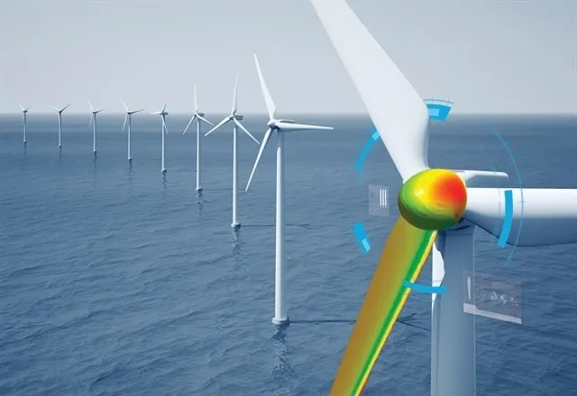
Blade-resolved CFD meshes the blade surface and its boundary layer, with a sliding or overset mesh for the rotation. It gives blade loads, stall, tip and root effects and the interaction with tower and nacelle, and its cost makes it a rotor tool, not a farm tool. An actuator line replaces the blade by a rotating line of body forces from tabulated airfoil data, an actuator disc by a loaded surface; only the rotating disc and the line capture wake rotation, and stall is an input, not a result.
How far to trust either is a measured question. The Mexnext-III final report (IEA Wind Task 29) compared over 20 codes, from blade-element momentum to CFD, with New MEXICO measurements on a 4.5 m rotor in a large wind tunnel. Design models proved accurate in uniform axial inflow and more scattered for the turbulent wake, separated flow and tip effects, and CFD results depend heavily on the many input and output choices. We fix those choices in a template, turbulence and transition treatment, mesh and time step near the tip, load post-processing, and record them with every run.
How do you simulate wake losses, blockage and atmospheric stability?
At farm scale the turbines become actuator models in a boundary-layer flow. Large-eddy simulation resolves the large eddies, and with them the meandering, but is sensitive to its subgrid and turbine-force models; the review puts it near 103–104 CPU hours per simulation against about 10−3 for an analytical wake model, six to seven orders of magnitude apart. RANS parametrises all turbulence scales and returns the mean wake.
Doubrawa and colleagues (2020) compared 13 approaches with lidar wake measurements at a research turbine: in the neutral benchmark performance followed model fidelity and LES did best, while in the stable case steady RANS did better, because non-canonical inflow is easier to prescribe and runs are cheap enough to repeat. They name inflow as a main challenge and trace differences among time-stepping models largely to wake meandering.
Stability therefore belongs in the boundary conditions. Wakes recover faster and meander more in a convective boundary layer than in a neutral or stable one. Under a strongly stratified free atmosphere, gravity waves deepen the induction zone ahead of a farm; the review cites actuator-disc results with the wind 2.5 rotor diameters upwind about 3% below the free stream. At Horns Rev, power falls to a minimum with the wind aligned to a row and recovers within about 10°. Over a ridge, superposing a flat-terrain wake on the terrain flow, standard in industry, is questionable even for moderate slopes.
- Induction zone ahead of the farm. The rotors take momentum, so the air slows and lifts before it arrives, and the effect accumulates over every row. It depends on layout, wind direction, spacing and thrust coefficient. The speed measured upwind is not the speed the first row sees, which a per-turbine wake model alone misses.
- Inversion lid and gravity waves. When the free atmosphere above the boundary layer is stably stratified, the farm's upward push can set up standing gravity waves. In subcritical flow they reach upstream, deepen the induction zone and lower the output of the first rows. The domain has to reach the inversion, with the stratification imposed.
- Wake and added turbulence. Behind each rotor sit a velocity deficit and extra turbulence, strongest near the top-tip level where the shear is highest. That turbulence is the fatigue input for the next rotor's blades, so one field feeds both the energy question and the structural one.
- Stable night, convective day. The same turbines, spacing and wind speed give a long, persistent wake in a stable boundary layer and a short, quickly mixed one in a convective layer, because the turbulence that refills the wake differs. Stability is a boundary condition to set per case, not a correction to apply afterwards.
- Ridge and pressure gradient. Over terrain a wake recovers faster where the pressure gradient is favourable, on the windward side, and slower where it is adverse, on the lee side, and lee separation lifts its path. Adding a flat-terrain wake to the flow over the hill misses both effects.
- Sheared inflow. Wind speed rises with height in a shape set by surface roughness and stability, and on a stable night a low-level jet can sit within the rotor height range. The shear loads each blade once per revolution and is the profile every model has to start from.
Which wind turbine question needs which model?
| Question | Model | What it reports | Limit to state |
|---|---|---|---|
| Blade loads, stall, tip and root effects | Blade-resolved URANS or hybrid RANS-LES | Surface pressure and shear, load history | One rotor, near wake |
| One wake and its turbulence | Actuator line or disc in LES, turbulent inflow | Deficit, wander, turbulence field | Blade stall is an input |
| Farm blockage, stability, farm-to-farm | Farm-scale RANS or LES | Induction, stability-dependent losses | Domain to the inversion, inflow data |
| Layout and yaw schedule | Calibrated wake model plus surrogate | Thousands of cases: mean deficit, deflection | Valid inside the calibrated range |
| Ridge and terrain siting | Terrain-following RANS or LES | Pressure gradient, separation, wake path | Terrain and roughness data |
| Blade structure under load | CFD loads mapped to FEA, one-way or two-way | Stress, deflection, fatigue input | Two-way if deflection changes loads |
How do aerodynamic loads reach the blade structure?
A blade is a flexible beam whose load depends on its own shape. CFD pressure and shear are mapped to the structural mesh by a conservative transfer, which keeps total force and moment although the meshes differ, and go to Abaqus or Nastran for stress, deflection and fatigue. One-way coupling suffices when deflection barely changes the aerodynamics; on long, flexible blades twist and bend change the angle of attack, so we close the loop two-way (see one-way FSI for fatigue and two-way FSI).
The wake is the fatigue input for the next blade: the review gives the added turbulence as ΔI = √(Iw2 − I2), peaking two to four diameters downstream at top-tip level. IEC 61400-1:2019 specifies design requirements for the structural integrity of wind turbines of all sizes. CFD enters where an engineering aerodynamic model is least certain: stall, the tip and wake interaction.
How credible is a wake simulation, and what do you validate against?
Verification is mesh and time-step convergence on thrust, power and the deficit at fixed stations, and for LES an averaging window long enough to converge. Validation uses measurements: the lidar benchmarks above, New MEXICO, your SCADA and wake data, and AWAKEN. IEC 61400-12-1:2022 specifies how to measure a single turbine's power performance and requires an assessment of uncertainty sources, which sets what the model is compared with. We sweep inflow turbulence, wake growth rate, roughness and thrust curve to a range.
A wake-loss prediction is not a yield guarantee
Where does AI help wind farm design, and where does it not?
- Layout and yaw optimisation. An engineering wake model is cheap enough for an optimiser; a surrogate trained on designed CFD or LES runs over speed, direction, turbulence and stability carries the corrections it misses.
- Wake-model calibration. An inverse fit of wake growth and deflection to lidar, SCADA or benchmark data by stability class returns a range, not one constant.
- Rotor loads. A surrogate of blade loads over inflow angle, tip-speed ratio and pitch gives the structural team a loads database; anything outside the sampled range goes to the full model.
It does not replace the field campaign, repair a wrong inflow or extrapolate: a surrogate trained on neutral flow says nothing about a stable night with a low-level jet, or a turbine with a different thrust curve. Fleming and colleagues (2019) measured about 14% more energy on the downstream turbine of a closely spaced pair over a 10° sector at a commercial farm, 4% for the pair, consistent with the engineering model that designed the controller, and list near-wake modelling, complex terrain and summer conditions as difficulties. The review adds that steering suits offshore or stable flow best, with blade loads under yaw still to be studied. See surrogate models for CFD and FEA and our surrogate modelling and uncertainty quantification pages.
From one wake study to a wind workflow you keep
The return comes when your engineers can put the next turbine type, site or layout through the same chain.
- Physics model. CFD and FEA set up once, as templates: geometry clean-up, mesh, solver settings and post-processing that every later run reuses.
- Validation. Mesh and time-step studies, and comparison with tests or full-scale data, so the model's uncertainty is known before it is trusted.
- Automated runs. Scripted runs over the parameters and operating conditions that matter, on your hardware or in the cloud.
- AI surrogate. A machine-learning model trained on those runs answers in seconds and says how sure it is; low-confidence questions go back to the solver.
- Decision tool. Optimisation, trade-off charts or operating guidance, in a form your engineers and operators use every day.
- Field data. Test, trial and monitoring data flow back to recalibrate the model, so it improves with every project instead of being rebuilt.
- A parametric rotor and farm model in your existing solver: blade geometry, pitch, rotor speed, layout and terrain as parameters, one template recording turbulence, mesh and time-step choices.
- An inflow library of precursor boundary-layer runs per stability class and roughness.
- A calibration script from your lidar, SCADA or benchmark data to wake growth and deflection parameters, with fit and range on record.
- A load-transfer post-processor writing pressure and shear to the structural mesh with a force and moment check.
- A validation record against your power curve and a wake measurement, tolerances set before the run.
- A surrogate with a stated range and a gate to the full model outside it.
- Handover and training, so your team runs and extends it. See our training and software development services.
Questions engineers ask about wind turbine CFD
Is blade-resolved CFD better than an actuator line model?
Can CFD replace a measurement campaign for wake losses?
How is atmospheric stability handled in a wake simulation?
Does wake steering work on every site?
What about floating wind and turbine noise?
If a layout freeze or blade design review is waiting on a wake or load answer, send us the rotor geometry or thrust and power curves, the site wind rose with any lidar, mast or SCADA data, the layout candidates and terrain, and the loads your structural team needs. We reply with the model chain we would set up for each question, its validation record and what a surrogate could cover. Start with a conversation, or read our wind turbine and farm page and wind turbine industry page.