Turbomachinery aeromechanics: finding blade flutter and forced-response risk before the rig does
Blades, blisks and impellers that pass aerodynamic design can still crack from high-cycle fatigue. How Campbell diagrams, flutter and forced-response analysis and mistuning checks catch it early, and how a surrogate with a solver gate brings those checks into optimisation.
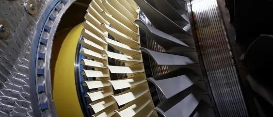
Turbomachinery aeromechanics is the engineering of making a blade, blisk or impeller survive the vibration its own aerodynamics creates, through resonance, flutter and forced response. A design that meets its efficiency and pressure-ratio targets can still crack from high-cycle fatigue (HCF) on the test rig, and the later that is found, the more it costs.
Picture the review after a strain-gauge campaign shows a blade row ringing inside the operating range, with tooling ordered. What is left is a redesign, a restricted speed range or a derate. Here is how to find that earlier, while changing the geometry is cheap.
Why do blades that pass aerodynamic design still crack in test?
Aerodynamic optimisation minimises loss and meets flow and pressure targets at a handful of operating points. The vibration problem lives elsewhere: in the natural frequencies of the blade-disk system, the unsteady forcing from neighbouring rows and inlet flow, and the small damping that sets the response. Reshaping a blade for a point of efficiency changes its mass, stiffness and loading together, so a frequency margin that was acceptable for the baseline is not guaranteed for the variant. Found after the optimisation, a failure means rerunning the loop; found on the rig, it means hardware, rig time and schedule.
A frequency margin is not an aeromechanical margin
How do Campbell diagrams and engine orders show resonance risk?
A Campbell diagram plots blade natural frequencies against rotor speed. Excitation from upstream wakes, vanes, struts and distorted inlet flow arrives at whole multiples of rotor speed, the engine orders: f = EO × N / 60. Where an engine-order line crosses a mode line inside the operating range, the blade can resonate.
- Mode lines. Natural frequency of each blade-disk mode against rotor speed. They rise a little with speed as centrifugal stiffening grows, and each mode family has one line per nodal diameter.
- Engine-order lines. Excitation at whole multiples of rotor speed, f = EO x N / 60: upstream wakes, vanes and struts, or inlet distortion. In a cyclic-symmetry model an engine order excites the travelling wave with the matching nodal diameter.
- Operating range. The speeds the machine must run at, steady and during transients. Only crossings inside it, or close to it, need a full forced-response assessment.
- Crossings. Resonances where an engine-order line meets a mode line. Whether one is dangerous depends on how well the forcing matches the mode shape and on the total damping, not on the crossing alone.
- Scatter bands. Geometry tolerance, wear, temperature and mistuning shift the frequencies, so each line is really a band and each crossing a region. This is where margins are spent.
- Flutter. Self-excited vibration needs no engine-order line. It appears when the aerodynamic work per cycle feeds more energy into the blade than the damping removes, usually at low reduced frequency in a torsion or first-bending mode.
- Nodal diameters. A bladed disk has one mode per nodal diameter in each family. For a cyclic-symmetric rotor, an engine order excites the travelling wave with the matching nodal diameter, so frequencies come from an interference diagram, not one number.
- Not every crossing is equal. The forcing must couple to the mode shape.
- Frequencies move. Temperature, centrifugal stiffening, tolerance and wear shift them, so each line is really a band.
What is blade flutter, and how is aerodynamic damping calculated?
Flutter is a self-excited instability: the blade's own motion creates unsteady pressure that does net work on it every cycle, so vibration grows with no external forcing. Two parameters organise it. The reduced frequency, k = ωb / V with b the semi-chord, compares the vibration period with the flow transit time. The interblade phase angle, σ = 2π · ND / N, sets how neighbouring blades move. Low reduced frequency, heavy loading near stall and transonic shocks are the classic troublemakers.
The usual route is the energy method. The blade is made to move in a chosen mode as a travelling wave at one phase angle, unsteady CFD gives the pressure, and the work over one cycle is integrated. If the fluid takes energy out of the blade, aerodynamic damping is positive; if it puts energy in and structural damping cannot remove it, that mode flutters. This one-way calculation is valid when the flow hardly changes the mode shape. For dense fluids or strong coupling, an eigenvalue formulation solves the coupled system and reads damping from complex eigenvalues.
In NASA's flutter analysis of a transonic fan (Srivastava et al., 2002) the energy-exchange method agreed with measurements, shock position and strength strongly affected stability, and the running blade shape under load changed the calculated damping. The unloaded CAD shape is not the shape that flutters.
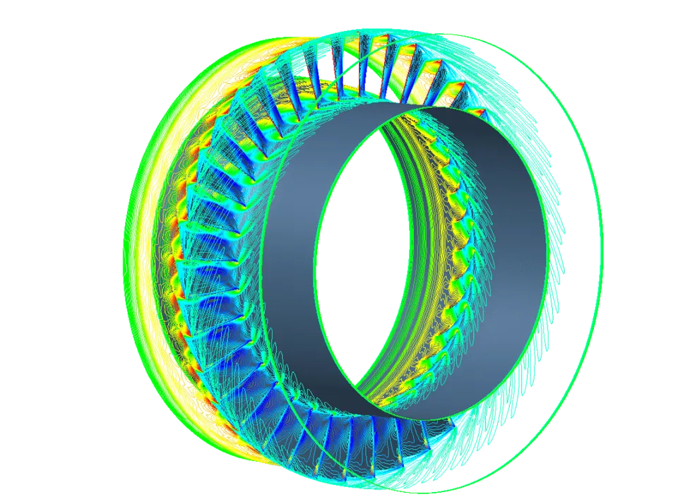
Forced response: wakes, distortion, and one-way versus two-way coupling
Forced response asks how large the vibration gets at a crossing. Forcing comes from the wakes and potential fields of neighbouring rows, from inlet distortion at low engine orders, and from off-design flow such as separation and rotating stall. Amplitude scales with modal force and inversely with total damping, so the flutter calculation's aerodynamic damping feeds straight in. Distortion shows what simplification costs: NASA Glenn's forced-response analysis of a distortion-tolerant fan with boundary layer ingestion (Min et al., 2018) used a full-rotor cyclic-symmetry model because single-blade models cannot capture the loading, and compared it with wind-tunnel data.
| Method | Where it fits | What it costs or misses |
|---|---|---|
| One-way: CFD forces into a structural response | Early design, many candidates, damping known from elsewhere | Damping is an input; blade-motion feedback is ignored |
| Two-way coupled (FSI) | Light structural damping, aerodynamic damping dominant, dense fluids | More setup and longer runs |
| Harmonic or nonlinear frequency-domain CFD | Periodic forcing, many engine orders and operating points | Fast, but shocks and separation need care and more harmonics |
| Time-marching, full annulus | Distortion, non-periodic flow, stall | The most expensive; kept for the cases that decide the design |
Our fluid-structure interaction work covers one-way and two-way coupling; the choice follows from how much of the damping is aerodynamic.
Mistuning, Goodman margins and where the uncertainty sits
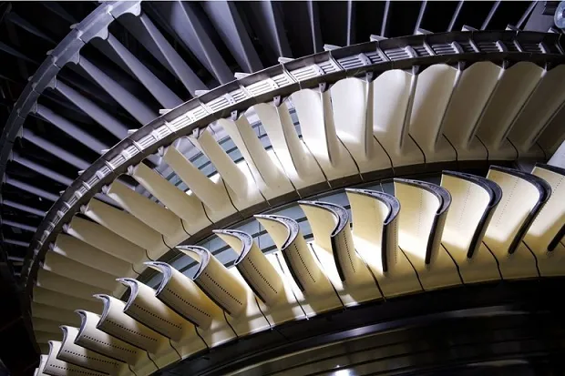
Real blades differ slightly in frequency, from tolerance, wear and material. That mistuning localises vibration, so a few blades respond far more than the tuned prediction. Whitehead's classic bound for a one-degree-of-freedom-per-blade model is an amplification of up to (1 + √N) / 2 for N blades, and blisks, which lack the friction damping of attached roots, are the sensitive case. NASA-sponsored report on the effects of mistuning on the forced response of turbomachinery rotors (Pierre, 1994) states that the amplification can be severe enough to cause blade failure. It can also help: in NASA contractor report on the influence of mistuning on blade torsional flutter (Srinivasan, 1980) a fan with slightly different blade frequencies was predicted stable in the cases studied, while the identical-blade system fluttered at a few phase angles.
Vibratory stress alone does not decide the outcome: fatigue strength depends on mean stress from centrifugal, gas and thermal loads. A Goodman or Haigh diagram plots allowable alternating stress against mean stress, and the margin is the distance from the predicted alternating stress, at the real mean stress, to that line, after knock-downs for temperature and surface. See our vibration fatigue simulation and durability and fatigue pages.
The uncertainty sits in four places, each a distribution, not a number:
- Geometry. Tolerance and the running shape move frequencies and shock position.
- Mistuning. Random, different for every rotor, so handled statistically.
- Damping. Aerodynamic, material and friction together: the least known input and the most powerful.
- Forcing. Wake depth, distortion amplitude and clearances, hardest to know before the rig runs.
The output should be a probability of exceeding the limit: see uncertainty quantification.
How can AI and surrogate models carry aeromechanical constraints into optimisation?
The aim is not to replace the solvers but to bring aeromechanics into the loop where thousands of candidates are judged. An optimiser needs every constraint as fast as its efficiency model; a CFD flutter run per nodal diameter per candidate is not.
- One parametrisation drives the CFD and the finite-element model through mesh morphing, so both stay in step.
- Designed experiments. Your solvers run a space-filling set across geometry and operating points, recording frequencies, aerodynamic damping per nodal diameter and modal forcing per engine order.
- Surrogates with uncertainty. Frequencies are the easiest, being smooth in the geometry. Damping near shocks and stall is the hardest.
- Constraints inside the optimiser. Efficiency, pressure ratio, mass and margin are traded together. See generative design and optimisation.
- Mistuning by sampling. Thousands of random patterns through a reduced-order model give a distribution of worst-blade response.
- A gate. A candidate outside the training range, uncertain, or close to a limit goes back to the solver, and the result joins the training data.
- Parametric geometry. One definition of the blade, blisk or impeller that drives both the CFD and the finite-element model, so aerodynamic and structural changes stay in step.
- Multi-objective optimiser. Trades efficiency, pressure ratio or flow range and mass against aeromechanical margin, which is a constraint and not a late check.
- Trained surrogate. Predicts frequencies, aerodynamic damping per nodal diameter and a forced-response metric in milliseconds, with an uncertainty estimate for every answer.
- Confidence gate. Keeps only answers that are inside the training range and carry a small predictive spread. Anything else is sent back to the solver.
- Solver check. Cyclic-symmetry modal analysis, CFD flutter by the energy method and harmonic or time-marching forced response: the physics that the surrogate imitates and answers to.
- Sign-off and learning loop. An automated Campbell and margin report, Goodman or Haigh checks and a mistuning study. Every solver result and test measurement returns to retrain the surrogate.
| Task | A surrogate can | The solver must |
|---|---|---|
| Frequencies and mode shapes | Return them in milliseconds across a parametrised family | Handle a new topology or boundary condition |
| Aerodynamic damping | Screen and rank candidates, with uncertainty | Decide cases near zero damping, shock jumps, stall, new regimes |
| Forced-response amplitude | Interpolate modal forcing between trained cases | Cover non-periodic distortion nobody trained on |
| Mistuning statistics | Make large sampling studies affordable | Replace the measured pattern of a real rotor |
| Sign-off | Automate the report and checks | Replace validated physics and test evidence |
Automating the post-processing is often the first step worth taking. A reusable template reads modal results per nodal diameter, the engine orders and the speed range, then writes the Campbell diagram, a crossing table with margins, damping per nodal diameter and the Goodman check for every candidate, whichever solver produced them. For the discipline around surrogates, see our article on surrogate models for CFD and FEA and reduced-order models.
From one aeromechanics study to a capability you keep
A single campaign answers one question for one design. The larger return comes when the setup becomes a workflow your team runs, so the next blade or operating question costs hours, not weeks, and every answer is judged the same way. That is how we build turbomachinery aeromechanics work.
- Physics model. CFD and FEA set up once, as templates: geometry clean-up, mesh, solver settings and post-processing that every later run reuses.
- Validation. Mesh and time-step studies, and comparison with tests or full-scale data, so the model's uncertainty is known before it is trusted.
- Automated runs. Scripted runs over the parameters and operating conditions that matter, on your hardware or in the cloud.
- AI surrogate. A machine-learning model trained on those runs answers in seconds and says how sure it is; low-confidence questions go back to the solver.
- Decision tool. Optimisation, trade-off charts or operating guidance, in a form your engineers and operators use every day.
- Field data. Test, trial and monitoring data flow back to recalibrate the model, so it improves with every project instead of being rebuilt.
- Templates for the geometry, the cyclic-symmetry model, the CFD setup and an automated Campbell and margin report.
- A validation record tying the models to your rig, strain-gauge or tip-timing data.
- Automated runs over the parameters and operating conditions that matter.
- A trained surrogate with a confidence gate and written limits of validity.
- Training and handover, so your engineers extend it themselves: our training and software development services.
Questions engineers ask about blade flutter and forced response
What is the difference between flutter and forced response?
Can CFD predict flutter reliably?
Do I need two-way FSI for forced response?
Can a neural network predict blade vibration stress?
What do you need from us to start?
Our turbomachinery design work spans turbines, pumps and compressors, heat transfer and generative design; see also gas turbine simulation. If a blade row, a Campbell diagram or a test finding is on your desk, send us the geometry and the question. You will get a plain assessment of which risks matter and which models answer them.