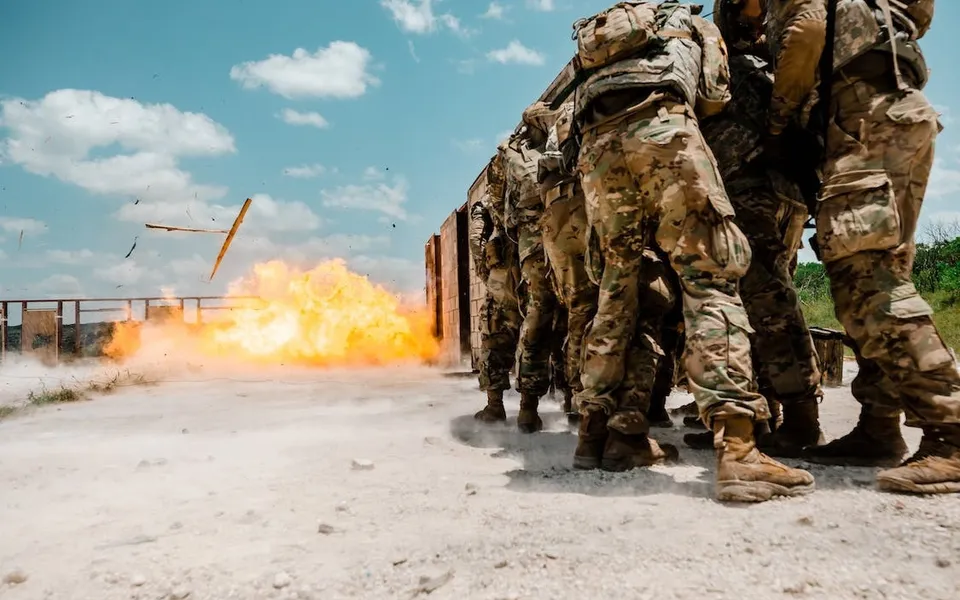
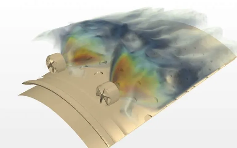
Vapour cloud explosion simulation for process area design loads
A congested, partly confined process area turns a gas cloud into a pressure load on walls, decks and supports. Explosion CFD, an exceedance curve and a mapped structural model turn that into a design accidental load your team can defend and rerun.
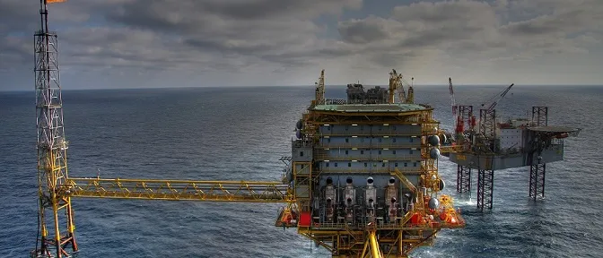
Vapour cloud explosion simulation predicts how a flammable cloud, ignited in a congested and partly confined process area, onshore or offshore, builds overpressure, and turns the pressure-time results into design loads for the walls, decks and supports that must withstand it. We build that chain around your existing explosion CFD and explicit FE solvers, so the design accidental load you defend at the review comes from a record your team can rerun.
The blast wall between the compressor module and the control room is on the drawing, and its design load is still a placeholder. Too high, and wall, supports and deck grow in steel, weight and schedule. Too low, and it may not do its job. The number has to survive an owner's, insurer's or regulator's questions, and the next layout change.
What does vapour cloud explosion simulation have to predict?
Flame speed decides the pressure. The TNO Yellow Book (CPR 14E, chapter 5, second print 2005) puts laminar flame speeds for normal hydrocarbons in the order of 5 to 30 m/s, too low for significant blast overpressure, so the cloud burns as a flash fire. Congestion supplies the missing turbulence: obstacles shed wakes into the expansion flow ahead of the flame, which raises the burning rate and drives a faster flow.
Geometry therefore sets the load. Roofs, decks and walls decide how fast the expansion can leave, and the open side is the vent. The Yellow Book calls “unconfined” a misnomer for these explosions, because partial confinement and obstruction produce the pressure. CFD earns its cost by resolving obstacles, confinement, ignition position and vent paths for your actual layout. See our oil, gas and petrochemical blast simulation and blast, explosion and fire pages for the wider capability.
- Ignition and the slow start. A flame that starts in a quiet cloud is laminar and slow. On its own it is far too slow to make damaging overpressure, and a cloud that never meets obstacles or confinement burns as a flash fire.
- Expansion flow ahead of the flame. Burning gas expands, so the unburned mixture is pushed ahead of the flame, past every obstacle and out of the open side. The faster the flame, the faster this flow.
- Obstacles and turbulent wakes. Pipes, vessels, trays and steelwork shed turbulent wakes into that flow. The model can only make turbulence at the obstacles it contains, so the congestion in the model is an input to the load.
- Flame speed feeds back. Turbulence raises the burning rate, a faster burn drives a stronger expansion flow, and the stronger flow makes more turbulence. The loop accelerates the flame while it stays in the obstacle field.
- Confinement and the vent path. A roof, deck or wall slows the expanding gas on its way out, and the open side is the vent. The same flame speed gives a higher pressure where the vent path is smaller, so confinement belongs in the geometry as much as the obstacles.
- Overpressure along the flame path. Pressure builds while the flame crosses the congested region and falls once it reaches open cloud, where combustion slows. A different layout moves and reshapes this curve, which is why the load is computed for the actual geometry.
Why is a gas explosion load so hard to pin down?
Because the inputs that matter most are the least certain: gas quantity, concentration, ignition position and the obstacles the flame meets. The HSE page on the Buncefield incident records explosions on 11 December 2005 at the Hemel Hempstead oil storage depot, with more than 40 people injured. In 2007 the Board's Explosion Mechanism Advisory Group wrote that the severe explosion “would not have been anticipated in any major hazard assessment” of the depot. Pipework congestion was largely absent, and entirely absent in some areas where high pressures arose; trees and undergrowth along a lane may have acted in its place. The group could not identify one scenario that explained every aspect.
A fuel depot is not a process module, but the lesson transfers: the load carries your assumptions about what burns and what obstructs. We put the congestion revision, cloud definition and ignition set under change control in the load-case file.
The geometry you leave out sets the load
How are explosion loads usually derived, and where does that break?
Early studies use the Multi-Energy method from the Yellow Book: each obstructed or partly confined region becomes a sub-explosion with a strength class from 1 to 10, where 10 is detonative, and the rest of the cloud burns out slowly. Without better guidance the Yellow Book advises class 10 for obstructed regions and calls that conservative. Blast is read from charts in scaled distance r′ = r / (E/pa)1/3, with E the combustion energy.
It ranks areas well and a specific wall poorly. The blast is symmetric around each region, and the Yellow Book says the method ignores directional effects, pointing to CFD for them. The IChemE Hazards 28 paper on structural design loads for blast reports a benchmark in which five consultants ran the same probabilistic explosion study for one platform: four predicted a 10−4 per year load of 0.5 to 1.1 barg and one about 2 barg, using steady state dispersion. Method choices, not just the solver, move the answer.
| Question | Method | What it gives | Where it stops |
|---|---|---|---|
| Which areas matter most? | Multi-Energy method | A symmetric blast from each obstructed region | No direction; class 10 is conservative by design |
| What load does this wall or deck see? | Explosion CFD on the actual layout | Pressure-time histories on monitor panels | Needs layout, cloud definition, grid practice |
| What is the design accidental load? | Probabilistic CFD scenario set with an exceedance curve | The load per panel at a stated frequency | Large run set; ignition and wind inputs move it |
| Does the structure carry that load? | Mapped loads on an FE model in LS-DYNA or Abaqus | Deflection, plasticity, support forces | One-way mapping treats the wall as rigid |
| Which rare scenarios set the tail? | Full CFD and FE reruns of the severest cases | Confirmation of what a screen ranked highest | Cost, so a screen comes first |
How do you get from pressure-time histories to a design accidental load?
The usual route is probabilistic. The Hazards 28 paper describes the Annex F procedure of NORSOK Z-013 (edition 3, 2010; the current edition is NORSOK Z-013:2024, Risk and emergency preparedness assessment) as CFD for ventilation, dispersion and explosion, and says ISO 19901-3 recommends it. A large scenario set, weighted by the frequency of each stage, gives an exceedance curve for each target, and the design load is read at the allowable frequency.
Each scenario i has a frequency fi: release frequency times the probability of that wind and that ignition. The frequency of exceeding p is F(p) = Σ fi over scenarios with peak pi ≥ p, and the design accidental load (DAL) is the p where F equals the allowable frequency. The owner, regulator or insurer sets that frequency. The simulation does not.
A pressure at one point is not the load on a structure. In the paper's FPSO blast wall, the 10−4 per year load of 2 barg applied only in one corner, beside a heavily congested high-pressure compression module; the side beside a lower-pressure separation module saw significantly less. Applying 2 barg across the wall was clearly overly conservative against the response computed scenario by scenario. On another target, the ignition model alone moved a 10−4 per year load from 2 barg to over 4.5 barg.
- Scenario set. Each dot is one scenario: leak size and direction, wind and ignition position. The few severe ones, in warning colour, shape the tail of the curve and are the first to be run again in full CFD.
- CFD cases. Dispersion builds the cloud, then the explosion run gives a pressure-time history on every monitor panel of the target. A congested module at high pressure drives the nearest panels hardest, and a lower-pressure module drives them less.
- Exceedance curve. The frequencies of the scenarios are added from the severest down, which gives the frequency with which each overpressure level is reached or exceeded at the target.
- Target frequency and the DAL. Where the curve crosses the allowable frequency, the design accidental load is read. The allowable frequency comes from the owner, regulator or insurer, not from the simulation.
- Load per panel. Reading the same frequency panel by panel shows where on the structure the load is high. A single worst-case value applied everywhere hides that pattern.
- Structural FE model. Each panel's pressure-time history goes to the matching elements, with its own arrival time. The CFD treats the wall as rigid, so a structure that deflects enough to change the venting needs a further check.
How do you map explosion CFD loads onto the structural FE model?
Keep the time history, not just the peak. Tie each CFD monitor panel to an element set, apply its pressure-time curve in LS-DYNA or Abaqus, and delay it by its arrival time. The paper compared one representative event applied everywhere at once, the same event delayed by the local speed of sound, and scenario-by-scenario coupling. For a fairly stiff wall they agreed reasonably, and the authors expect the agreement may diminish for less stiff structures. A history matters because of the single-degree-of-freedom equation m d2x/dt2 + c dx/dt + kx = p(t)A: a load short against the natural period T = 2π√(m/k) drives the response through its impulse, a long one through its peak.
Two cautions. One-way mapping treats the structure as rigid in the CFD, so a wall that deflects enough to change the venting needs a further check, and the explicit model needs the energy, mass-scaling and contact checks from our article on a crash model you can trust. And CFD and structural teams often work apart; the paper calls that interface often primitive. A mapping script and a shared load-case file close it.
Where does AI help vapour cloud explosion analysis, and where does it not?
- Screening and sensitivity. A surrogate trained on a planned CFD run set predicts panel peak pressure and impulse from release rate, wind, ignition position and cloud size, inside the layout's range. The team can change the ignition model or the release frequencies and watch the exceedance curve move without a new CFD campaign. See surrogate models for CFD and FEA.
- Adaptive run planning. New CFD runs go where the severest outcomes sit, so the tail that sets the design load is sampled most densely.
It does not replace the physics at the tail. A surrogate trained on one layout knows nothing about another module or a changed wall, and it inherits every error of the CFD behind its data. The scenarios that set the design load are re-run in full CFD and FE, and the surrogate carries a stated range and a gate that sends anything outside it to the full model. See validation and uncertainty for AI surrogate models.
What does the simulation not replace?
It supports the design decision and does not make it. Nothing we build certifies, rates or approves a facility, replaces the explosion risk assessment, testing, code compliance or competent-person sign-off, or guarantees that a structure survives. Whether virtual evidence is accepted, against which frequency and criteria, is agreed with the authority and the owner's process-safety function before the study.
From one explosion study to a capability you keep
The return comes when your engineers can re-run the chain after a module moves, not work from a stale report.
- Physics model. CFD and FEA set up once, as templates: geometry clean-up, mesh, solver settings and post-processing that every later run reuses.
- Validation. Mesh and time-step studies, and comparison with tests or full-scale data, so the model's uncertainty is known before it is trusted.
- Automated runs. Scripted runs over the parameters and operating conditions that matter, on your hardware or in the cloud.
- AI surrogate. A machine-learning model trained on those runs answers in seconds and says how sure it is; low-confidence questions go back to the solver.
- Decision tool. Optimisation, trade-off charts or operating guidance, in a form your engineers and operators use every day.
- Field data. Test, trial and monitoring data flow back to recalibrate the model, so it improves with every project instead of being rebuilt.
- A parameterised layout and scenario matrix in your explosion CFD solver, with releases, wind, ignition positions and the congestion revision in a load-case file.
- An automated run set that submits cases, extracts monitor-panel histories and rejects runs that fail the checks.
- An exceedance builder that adds scenario frequencies, reads the load per panel at the allowable frequency and shows how the curve moves when an assumption changes.
- A mapping tool that applies panel histories, with arrival times, to the structural model in LS-DYNA or Abaqus, with the energy, mass and contact checks.
- A validation record against the experiments and benchmarks you hold, with the spread from unmeasured inputs.
- A surrogate with a stated range and a gate, plus handover and training so your team extends it. See our training and software development services.
Questions engineers ask about vapour cloud explosion simulation
What is a vapour cloud explosion?
What is a design accidental load?
Is the Multi-Energy method enough, or do I need CFD?
Can simulation replace explosion testing or the risk assessment?
What do you need from us to start?
If a blast wall load is holding up a layout freeze, send us the module layout or a description of it, your current load basis with its target frequency, the structure and its FE model if one exists, and your solvers. We will reply with how we would build the scenario set and checks, what the validation record should hold, how loads would map onto your structural model, and where a surrogate would help and where its range would end. Start with a conversation.