Acoustic liner design for turbofan engines, from duct modes to certified noise
A liner absorbs the duct modes a fan generates, in the flow the engine runs. Designing it against the real source, a validated impedance model and the certification metric settles depth, porosity and segment layout before nacelle tooling is frozen.
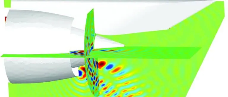
Acoustic liner design sets the facesheet and cavity of the honeycomb panels that line a turbofan nacelle so that they absorb the duct modes the fan actually generates, at the frequencies and flow speeds the engine runs. We build that design chain around your existing CFD, finite element and duct-acoustics solvers, Actran among them, so liner impedance, segment layout and certification noise are settled before nacelle tooling is frozen.
The first fan rig test shows a blade-passing tone above the noise budget, and the lined configuration removes less than the model promised. The liner was specified from a previous engine's spectrum, and every option now costs weight, length or schedule. The review asks which modes the fan puts into the duct, what impedance they need, and whether the liner presents it in the flow it will see.
What is an acoustic liner, and why is turbofan noise hard to treat?
The most common treatment in modern turbofan inlets and bypass ducts is a resistive facesheet resonator: a perforated sheet over a honeycomb core over a solid backing. Berton at NASA Glenn (22nd AIAA/CEAS Aeroacoustics Conference, 2016) reports that facesheet porosity sets the level of the absorption peak, cavity depth sets its frequency, and up to three layers widen the band. To first order the cavity contributes a reactance of magnitude cot(kh), which passes through zero at kh = π/2, a depth of a quarter wavelength; the facesheet adds resistance and mass. The surface has an impedance, Z / (ρ0c0) = R + iX: pressure over normal velocity at the wall.
Inside the duct the sound is not a plane wave but a sum of modes, each a pattern ψ(r) ei(mθ + kxx − ωt) with circumferential order m. For a hard wall and a uniform axial Mach number M, the axial wavenumber is kx = k [−M ± √(1 − (1 − M2)(κ/k)2)] / (1 − M2), with k = ω/c and κ the radial eigenvalue of the mode. It propagates only where its cut-off ratio, k / (κ√(1 − M2)), exceeds 1; below that it decays and never reaches the far field.
Tones are set by geometry. Koch at NASA Glenn (Noise-Con 2023) combines duct theory with the Tyler and Sofrin relation: wakes from B rotor blades meeting V stator vanes create circumferential orders m = nB + kV at the n-th blade-passing harmonic, for every integer k. Each order spins at n B Ω / m, and only those above cut-off propagate, so blade and vane counts decide which tones exist in the duct.
- Rotor wakes. Each of the B blades leaves a wake, so the stator meets B wakes per revolution: the blade-passing frequency is B times the shaft speed, and its harmonics n = 2, 3 follow.
- Stator vanes. The V vanes turn the wake flow into a pattern that repeats V times around the annulus. The vane count is a design choice, and it decides which circumferential orders the interaction can create.
- Spinning mode. Each order m is a pattern that turns round the duct at n B Ω / m for rotor speed Ω; orders of opposite sign turn in opposite directions. The liner has to absorb this pattern, not a plane wave.
- Mode lattice. The Tyler-Sofrin rule m = nB + kV lists every order the rotor-stator interaction can create at the n-th blade-passing harmonic, one for each integer k. Each dot is one such order.
- Cut-off boundary. Every order has a frequency below which it is evanescent and decays along the duct. These frequencies grow with the order, which draws the V: higher harmonics sit higher up it, so more orders can propagate.
- Cut-on orders. Dots inside the V travel along the duct, meet the liner and radiate. A vane count that leaves few or none inside at the speeds that matter is a design choice worth making before treatment; the liner works on what remains.
Engine trends move the target. Parrott, Jones and Watson at NASA Langley (Noise-Con 2005) describe how rising bypass ratio and shorter nacelles cut the lined length relative to duct diameter, lower the tonal spectrum and raise the share of broadband noise, so a liner must absorb a wider band over less wall. Certification counts what the ground hears: Berton explains that the metric is effective perceived noise level at three measurement points, with a tone penalty highest between 500 and 5000 Hz.
How is a turbofan liner designed today, and where does that break?
The established route, as NASA's DGEN inlet-liner study (Sutliff, Nark, Jones and Schiller) lays it out, has four steps. A duct-propagation code predicts the optimum impedance spectrum for a source and flow condition. Liner models find the geometry, within manufacturing limits, closest to it. The code predicts the attenuation, and the loop iterates. With no source data at the start, NASA drove it with a statistical source model.
Three things break it. First, the source. Low, Premo and Yu in a Pratt & Whitney, Boeing and Rohr liner design report for NASA (NASA/CR-20220015374) write that the major difficulty, whichever method a team chose, was the lack of knowledge of the hardwall fan source's modal structure, and that liners for new engines are commonly designed before measured hardwall spectra exist. They list five approximate descriptions of modal energy, and the optimum impedance follows the estimate.
Second, the impedance. Parrott and colleagues write that it is a property of the liner alone only if the surface is locally reacting, linear and insensitive to grazing flow; perforate-over-honeycomb liners are none of these, so the boundary condition describes liner and flow together. For a validation liner, educed impedances departed from a first-principles prediction by up to 0.5 ρc, away from the anti-resonance, as centreline Mach number rose to 0.5, in part from uncertainty about which flow parameter to use.
Third, the hand-offs. The grazing-flow condition in common use, Ingard-Myers, treats the flow at the liner as a vortex sheet, and NASA's own stability analysis notes that it is subject to a Kelvin-Helmholtz instability, which is why modified forms exist. Which form a solver applies, and whether the real boundary layer is thin enough for it, is a check, not a default. Found after tooling, a wrong impedance costs recut cores or lost margin.
How do you simulate acoustic liner performance in a nacelle?
We build the chain in six stages, with a check at each hand-off.
- Mean flow. CFD in Ansys Fluent, Siemens STAR-CCM+ or your solver gives Mach number and boundary-layer thickness along the lined wall at each operating point. Check: wall pressure and boundary-layer data from rig or engine.
- Source. Unsteady CFD of the rotor wakes gives the tone excitation, and the Tyler-Sofrin orders say which propagate. Broadband noise gets a stated modal-energy model. Check: rotating-rake mode data, or far-field arrays.
- Duct propagation and radiation. A finite element duct-acoustics model, Actran for example, carries each mode through the lined and hard-wall segments, scatters energy between modes at every impedance step, and radiates to the far field. Check: the hardwall case first, then the lined case, against rig attenuation.
- Liner impedance. A transmission-line model along each cell with a lumped element across the perforate, as in the DGEN work, turns porosity, hole size, depth and septa into impedance. On the measured side, eduction iterates a finite element field model against rig pressures; at Langley, 95 fixed microphones. Check: the sound levels and flow speeds the engine will run.
- Panel and installation. Core depth, mass and panel stiffness, in Abaqus or Nastran, limit the impedance that can be built and enter the optimisation as constraints.
- Certification. The radiated field goes through flight path, propagation and tone-corrected perceived noise at the three measurement points. Berton's method works backwards from that metric to the ideal attenuation spectrum, then looks for the liner that matches it.
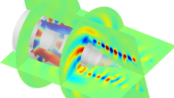
- Fan source. Rotor wakes and the stator create the duct modes of the first diagram. Tones sit in a few orders, broadband noise spreads over many. The modal content is the least certain input, so it enters as a stated, bounded assumption.
- Hard wall and grazing flow. Flow runs along the wall past the liner, towards the fan in an inlet and so against the sound. Its Mach number and boundary layer change how modes propagate and how the liner behaves; CFD supplies the mean flow at each operating point.
- Liner cell. Perforated facesheet, honeycomb cavity and backing, as in the zoomed cell. Porosity sets the level of the absorption peak and depth its frequency; a septum adds a second layer. Flow through the holes is nonlinear, so the impedance R + iX depends on sound level and grazing flow and is fitted to eduction data.
- Attenuation along the liner. Each mode loses energy along the lined wall at its own rate, set by impedance, flow and mode order. A short nacelle leaves less length for the liner to work in.
- Impedance steps scatter modes. Where the wall changes from hard to lined and back, energy is redistributed between modes. A finite element duct model captures this; a model that follows a single mode cannot.
- Radiation to the far field. What leaves the lip radiates with a directivity set by the modes that survive. That field is carried to the certification observers, and the perceived noise there is what the design is judged on.
- Geometry to spectrum. Cavity depth slides the absorption peak along the frequency axis, porosity changes its height, and extra layers widen the band. The optimiser works back from the spectrum the certification metric asks for to the geometry.
Where does AI help acoustic liner design, and where does it not?
- A surrogate of duct attenuation over resistance, reactance, frequency, Mach number and the modal-source set, trained on planned duct-solver runs, so multi-layer liners can be optimised against a certification metric. See surrogate models for CFD and FEA.
- Calibration of the impedance model. Jones, Parrott and Watson (14th AIAA/CEAS Aeroacoustics Conference, 2008) found the discharge coefficient the major contributor to uncertainty in the predicted impedance of the perforate-over-honeycomb liner they studied. We fit such parameters to eduction data with a Bayesian method that returns their uncertainty. See AI surrogate models you can sign off.
- Source inversion. Modal amplitudes inferred from in-duct or far-field arrays give a source distribution with its spread, not a hand-picked assumption.
Where it does not help: a surrogate does not know your engine's source, and it does not extend the physics beyond the levels, flow speeds and frequencies its data covered; a perforate whose resistance changes with level and flow is where extrapolation fails first. So it carries a stated range, and anything outside it goes back to the duct model.
Which model answers which liner question?
| Decision | Model | Needs | What it cannot tell you |
|---|---|---|---|
| Which orders can propagate at blade passing and its harmonics? | Cut-off analysis with the Tyler-Sofrin rule | Blade and vane counts, duct radii, speed, Mach number | Amplitudes: only which orders exist |
| What impedance should the liner present? | Duct propagation with an optimiser and bounded source models | Mode set, flow Mach number, treated length | Whether the source matches the assumption |
| Which facesheet and cell geometry gives that impedance? | Impedance model fitted to eduction data | Porosity, hole size, depth, level, flow | Behaviour outside the tested level and flow window |
| How much does the lined nacelle attenuate and radiate? | Finite element duct acoustics, mean flow, impedance segments | CFD mean flow, source, segment layout | Source level, if the source was assumed |
| Does the liner move the certification result? | System noise chain from radiated field to perceived noise | Directivity, flight paths, tone content | Installation effects outside the model |
| Is the built liner the one that was designed? | Impedance eduction on rig data | The panel in a grazing-flow rig, wall pressures | Curvature, splices and bond effects in the engine |
Do not optimise a liner against one assumed source
From one liner study to a liner design capability you keep
The return comes when your team runs the chain for the next fan or liner family.
- Physics model. CFD and FEA set up once, as templates: geometry clean-up, mesh, solver settings and post-processing that every later run reuses.
- Validation. Mesh and time-step studies, and comparison with tests or full-scale data, so the model's uncertainty is known before it is trusted.
- Automated runs. Scripted runs over the parameters and operating conditions that matter, on your hardware or in the cloud.
- AI surrogate. A machine-learning model trained on those runs answers in seconds and says how sure it is; low-confidence questions go back to the solver.
- Decision tool. Optimisation, trade-off charts or operating guidance, in a form your engineers and operators use every day.
- Field data. Test, trial and monitoring data flow back to recalibrate the model, so it improves with every project instead of being rebuilt.
- A parameterised nacelle-to-liner chain in your existing solvers, with facesheet, cell depth, septa and segment boundaries as parameters and the hand-off checks scripted.
- An impedance record: eduction data per facesheet and core, and the model parameters fitted from them with their uncertainty.
- A bounded set of source assumptions, re-run on every design and replaced by measured data as it arrives.
- A surrogate with a stated range over frequency, Mach number, impedance and modal set, with a gate that returns out-of-range requests to the duct model.
- Handover and training for your engineers. See our training and software development services.
Questions engineers ask about acoustic liners
How does an acoustic liner reduce engine noise?
What is liner impedance, and why does grazing flow change it?
Why do tones and broadband noise need different treatment?
Can a liner be designed without a measured source?
What do you need from us to start?
If a nacelle or fan rig is on your desk, send us the duct geometry, the blade and vane counts with speed lines, the liner definition by segment, the hardwall and lined noise data you hold, and any eduction measurements. We will reply with how we would build the chain, which source assumptions we would bound, which measurement would calibrate the impedance model and what the first attenuation map would let you decide. Start with a conversation, or read about our acoustics in aerospace engineering and aeroacoustics work, the acoustics and vibration section and rotor noise.