Transonic CFD simulation for wing drag, shock position and buffet onset
Your solver gives a drag increment you trust and a buffet-onset angle that moves with the turbulence model. Mesh families, drag decomposition and fine angle-of-attack sweeps show what is converged, what is model-form spread and what still needs a tunnel or flight point.
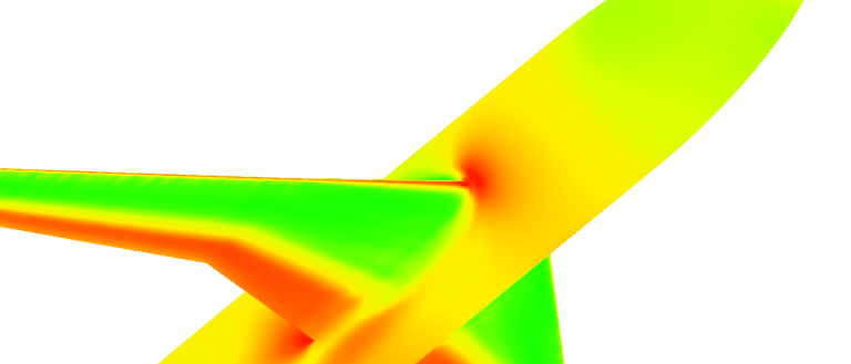
Transonic CFD simulation predicts the lift, drag, pitching moment and shock position of a wing where part of the flow is supersonic, and shows where the shock begins to separate the boundary layer and the wing buffets. We build it around your existing solver: a mesh family with a convergence record, a defended turbulence-model choice, drag split by physical part, automated envelope sweeps and a surrogate with a stated range.
The tunnel entry is booked and the wing and nacelle layout is close to freeze. Your solver gives a drag increment you trust and a lift-curve break you do not: change the turbulence model and the buffet-onset angle moves. Which number goes into the loads database, and which corner of the envelope still needs a tunnel run or a flight-test point? A wrong guess costs a tunnel slot or a late wing change.
What makes transonic CFD simulation hard?
Over the upper surface the flow accelerates past Mach 1 and returns to subsonic through a shock. Across a normal shock p2/p1 = 1 + 2γ(M12 − 1)/(γ + 1), and for a weak shock the entropy rise grows as the cube of (M12 − 1). A small error in the Mach number ahead of the shock becomes a large error in wave drag, and a misplaced shock shifts lift and pitching moment.
The shock also meets the boundary layer. Its pressure rise thickens the layer, and separation moves the shock back. Near buffet that loop is unsteady and self-sustained, so a steady solution may not describe the flow. NASA's Common Research Model (CRM), a transport wing designed for Mach 0.85, a lift coefficient of 0.50 and a Reynolds number of 40 million per reference chord, builds this in on purpose: the sixth workshop's report says its outboard pressure recovery is made aggressively adverse over the last 10 to 15% of local chord, to promote separation just above design lift.
- Supersonic pocket. Over the upper surface the flow accelerates through Mach 1. The dashed line is the sonic line and the shaded pocket under it is supersonic. Its size follows Mach number, lift and section shape, and it limits how strong the shock at its end can become.
- Shock. The pocket ends in a nearly normal shock: the pressure jumps and the entropy rises, which is wave drag. Its position sets the lift and pitching moment of the section, so a shock placed a little wrong in the model is a loads error. The drawing alternates between two shock positions.
- Boundary layer and separation. The shock's pressure rise thickens the boundary layer. With the shock aft the layer stays attached apart from a small bubble at its foot; with the shock forward it separates from the foot to the trailing edge. Where and how early this happens is what turbulence models disagree about.
- Upstream disturbances. Pressure disturbances from the trailing edge travel forward through the subsonic flow outside the pocket and move the shock, which changes the separation, which changes the disturbances. Near buffet this loop is self-sustained and unsteady, so a steady solution may not settle and unsteady runs are needed.
- Pressure distribution. Suction on the upper surface forms a plateau and jumps back at the shock; the area between the upper and lower curves is the lift. The shaded band is the spread of shock position: each solution can be valid on its own, yet the spread between models grows as the angle of attack rises.
- Lift-curve break. Lift rises in a straight line with angle of attack until separation grows, then falls away from that line. The angle at which it breaks is one working definition of buffet onset. It depends on turbulence model and mesh, and it is not the flight buffet boundary.
How accurate is CFD for wing drag prediction?
The AIAA Drag Prediction Workshops answer with common geometry and shared grid families. In the sixth, the bulk of the wing-body solutions at Mach 0.85, lift coefficient 0.5 and Reynolds number 5 million extrapolated to a continuum drag within a band 5 to 10 counts wide, a count being 0.0001 of CD, and most predicted the nacelle-pylon increment within the tunnel's 22.8 ± 1.2 counts. The report recalls a 270-count spread at the first workshop, on a different wing-body, and 41 counts at the fourth, one outlier excluded.
Off design is harder. Between 2.5 and 4.0 degrees angle of attack, 21 solutions (outliers removed) fanned out to a lift-coefficient spread of 0.063 and a pitching-moment spread of 0.045 at 4 degrees. Every turbulence model, grid scheme and solver loaded the aft wing more than the test did, and the authors ask whether steady RANS is adequate or URANS or detached-eddy simulation is needed. DLR's account of the seventh workshop (June 2022), built around shock-induced separation, again finds lift above and pitching moment more negative than the test. Design-point drag is a verified number; the buffet boundary is an estimate with a spread.
Which turbulence model for shock-induced separation?
None carries it alone. The sixth workshop ran 21 Spalart-Allmaras (SA) variants, 15 SA with the quadratic constitutive relation (QCR), 8 SST and others. Premature separation in the wing-body corner, absent from the tunnel data, appeared in most SA and SST solutions and was sensitive to grid detail; SA-QCR removed it, as did several other closures. In DLR's seventh-workshop runs SA-neg separated suddenly at 4 degrees, which DLR attributes to the one-equation model ignoring anisotropic stress in the corner flow; the Reynolds-stress model instead moved the outboard shock further upstream and gave a stronger pitch break. At the grid-convergence condition (Mach 0.85, Reynolds number 20 million, lift coefficient 0.58) the three models agree closely: continuum drag from 269.9 to 274.6 counts.
We choose by the decision. Attached cruise and increments: RANS with SA or SST on a converged mesh family. Shock position and buffet onset: SA-QCR or a Reynolds-stress closure beside a second model, plus unsteady runs to test whether the flow stays steady. The model spread is reported as model-form uncertainty, not averaged away.
| Question | What carries it | What it reports | What it cannot tell you |
|---|---|---|---|
| Cruise drag and increments | Steady RANS, fixed lift, mesh family | Drag by physical part, increment | Absolute drag to a count |
| Drag rise with Mach number | Mach sweep at fixed lift | Wave-drag share, drag-divergence trend | Separated off-design flow |
| Shock position and loads | Two or more turbulence models | Pressure at span stations, section loads | Which model is right at high alpha |
| Buffet onset | Fine alpha steps, QCR or Reynolds-stress, unsteady check | Lift break, separation extent | Flight buffet envelope |
| Tunnel-to-flight scaling | Reynolds sweep, corrections in the model | Reynolds increment, deformed shape | Tunnel interference itself |
How do you make mesh convergence and drag decomposition defensible?
Start with a refinement family, not one mesh: the workshop families grow in controlled steps through six levels (7 to 208 million cells in the sixth workshop's common grids), keep wall spacing at y+ of about 1 and keep every feature line. Plot drag against N−2/3, N being the unknowns; for a second-order scheme the intercept of a linear fit estimates the continuum. Structured families extrapolated to within 2 to 3 counts, unstructured to a 6 to 8 count spread. Run at fixed lift: the cases trim angle of attack to CL = 0.5 ± 0.0001, because drag at unequal lift is not comparable.
Then split the drag. Surface integration gives only pressure and friction drag, and numerical dissipation adds a spurious part that vanishes only on grids nobody can run. Paparone and Tognaccini (ICAS 2002) break drag into viscous and wave components from the entropy change and isolate the spurious part, making drag weakly dependent on mesh size. The wave share shows whether a change helped the shock or only the skin friction. For polars, plot CD − CL2/(πAR) as the workshop does, so lift dependence drops out and count-level differences show. Flux scheme and limiter go in the template: dissipation sets shock sharpness and spurious drag.
How do wind-tunnel results translate to flight?
The sixth-workshop report lists walls, support sting, tripped transition, aeroelastic deformation and corrections against a free-air, rigid, fully turbulent CFD model, and believes force and moment data differ between tunnels mainly through the corrections applied. The seventh workshop swept Reynolds number from 5 to 30 million at fixed lift against the CRM's design value of 40 million; DLR reproduces the expected lift gain and agrees better with the tunnel data that carry a sting correction. Aeroelastic twist of a little over one degree near the tip shifted transonic pressures significantly at model scale, and full-scale deformation can be an order of magnitude greater. So we compare as the workshops do: same conditions, the deformed shape for each angle (a coupled step; see our fluid-structure interaction page), increments rather than absolute forces, every correction on record.
A buffet-onset prediction is not a buffet envelope
Where does AI help an aerodynamic database, and where does it not?
An aerodynamic database feeds loads and flight mechanics across Mach number, angle of attack and control deflections. NASA's CFD Vision 2030 study calls CFD the primary source of aircraft load distributions and a growing source of performance databases, with tunnel data often only anchoring it at a few points. A surrogate earns its place there: a space-filling design of full runs and a held-out test set. The AIAA Applied Aerodynamics Surrogate Modeling group's open benchmark is the honest reference: its CRM case holds 149 RANS solutions over six parameters (Mach number 0.5 to 0.88, angle of attack, four control deflections), 105 for training and 44 for testing; the authors' own proper-orthogonal-decomposition example is accurate at benign conditions and deteriorates significantly once shocks are present.
So the surrogate is built with limits. It answers only inside the sampled envelope; sampling is refined along the lift-curve break the fine sweeps find; error is reported by region against held-out full runs; and any query outside the range or near the boundary goes back to the physics model. It does not predict buffet amplitude, extrapolate in Mach number or replace the solver as evidence. See surrogate models for CFD and FEA, AI surrogate models you can sign off and our uncertainty quantification page.
- Envelope and sweeps. Mach number runs across and lift, or angle of attack, up. A Mach sweep at fixed lift traces the drag rise; an angle-of-attack sweep climbs towards the boundary in steps that get finer where separation begins. Both are scripted, so every corner of the map is run the same way.
- Full CFD runs. Each dot is one converged run of the physics model, placed by a space-filling design so the sampled region has no large holes. Runs are checked for convergence and, near the boundary, for unsteadiness before they enter the database.
- Buffet-onset boundary. The lift break found by the fine sweeps, drawn as a curve inside a band. The band is the spread between turbulence models and meshes, which is reported, not hidden. Extra runs, the warm dots, are added along it because the response is not smooth there.
- Surrogate range. The dashed outline is where the surrogate may answer: inside the sampled region and clear of the boundary. Its error is measured against full runs held out of training, region by region, and stated with the range.
- Gate. A query outside the outline, or too close to the boundary, is not answered by the surrogate. It goes back to the full model, and its result joins the database.
- Test anchors. Wind-tunnel and flight-test points, one at cruise, are where the model is compared with measurement and every tunnel correction is on record. They anchor the database; neither the solver nor the surrogate replaces them.
From one wing study to an aerodynamic database you keep
The return comes when the next wing or flap setting goes through the same chain.
- Physics model. CFD and FEA set up once, as templates: geometry clean-up, mesh, solver settings and post-processing that every later run reuses.
- Validation. Mesh and time-step studies, and comparison with tests or full-scale data, so the model's uncertainty is known before it is trusted.
- Automated runs. Scripted runs over the parameters and operating conditions that matter, on your hardware or in the cloud.
- AI surrogate. A machine-learning model trained on those runs answers in seconds and says how sure it is; low-confidence questions go back to the solver.
- Decision tool. Optimisation, trade-off charts or operating guidance, in a form your engineers and operators use every day.
- Field data. Test, trial and monitoring data flow back to recalibrate the model, so it improves with every project instead of being rebuilt.
- A wing-body template in your existing solver, for example Ansys Fluent or Siemens Star-ccm+: deformed shape per angle, mesh family, flux scheme and fixed-lift trimming as one setup.
- A run manager for polars, Mach and Reynolds sweeps and fine angle-of-attack steps, with convergence and unsteadiness checks.
- A post-processor writing lift, drag by physical part, pitching moment, span-station pressure, separation extent and shock position per run.
- A validation record: your solver against the open workshop cases first, then your tunnel data with every correction written down.
- A surrogate with a stated range and a gate to the full model outside it.
- Handover and training, so your team runs and extends it. See our training and software development services, and the aerospace and defence page.
Questions engineers ask about transonic CFD
What is a drag count, and how accurate is CFD drag?
Is RANS enough for buffet?
Why do CFD and wind-tunnel drag differ?
Can a surrogate predict transonic shocks?
Can simulation be used for buffet certification?
If a drag number, a buffet-onset angle or an aerodynamic database is waiting on a transonic answer, send us the wing and body geometry with any deformed shapes, the Mach, Reynolds and lift conditions that matter, the tunnel or flight data and corrections you hold, and the solver and turbulence model you run now. We reply with how we would build the mesh family, model comparison and sweeps, and what the validation record and a surrogate could cover. Start with a conversation, or read the aerodynamics simulation page.