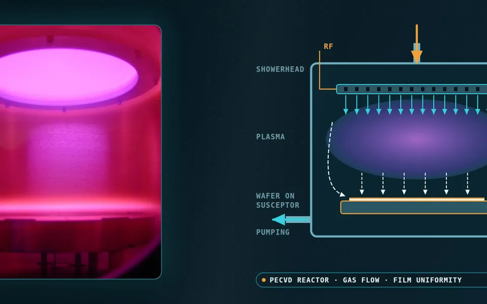
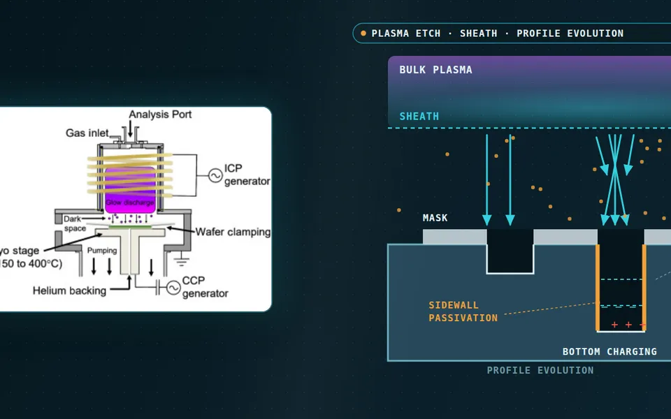
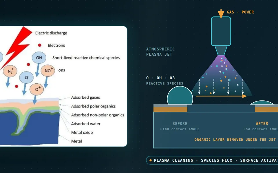
Plasma nanoparticle synthesis simulation for size control and reactor scale-up
The pilot reactor makes powder with the right mean size and the wrong coarse tail, and every fix costs a run and a round of microscopy. Coupled plasma, flow and aerosol models show how quench, power and flow set the size distribution.
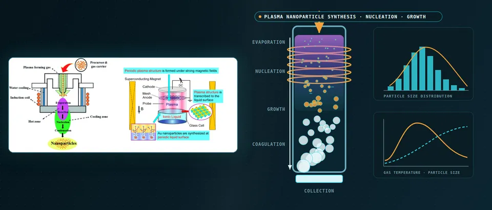
Plasma nanoparticle synthesis simulation links the plasma and gas flow, which fix the temperature and charge history of each parcel of vapour, to an aerosol model of nucleation, condensation, coagulation and charging, which turns that history into a size distribution. We build the chain around your reactor and your existing solver, validate it on your powder data, and hand over a surrogate with a stated range.
The pilot reactor's powder is on the microscope: mean size right, coarse tail wrong. Every fix is a run, then another round of imaging. The lever is large. In an induction-plasma silicon experiment, Shigeta, Hirayama and Ghedini (2021) measured a mean diameter of 150 nm with a standard deviation of 82 nm; an argon quench stream aimed at the plasma axis gave 27 nm and 9 nm, from about 1,200 particles counted on micrographs. That is not tuned by trial: it needs a model of the vapour's temperature history and what that history does to the distribution.
What sets the size distribution in plasma nanoparticle synthesis?
In a thermal plasma the heavy species reach around 10,000 K and particles form in the tail, where the gas cools steeply. With supersaturation S = pv/psat(T), the classical nucleation barrier is ΔG* = 16πσ3v12/[3(kT ln S)2], with σ the surface tension and v1 the monomer volume, and it sits in the exponent of the rate. Nucleation switches on over a narrow temperature window, and a ten per cent error in σ is a thirty-three per cent error in the barrier. Condensation then depletes the vapour; while liquid and hot, particles coagulate.
Cooling rate decides the race. A fast quench makes many nuclei at once and exhausts the vapour before they grow; a slow one makes fewer, which grow and coagulate for longer. The same study computed 18 cooling rates from 2.0 × 10³ to 6.4 × 10⁴ K s−1: a mean of 149.5 nm at 3.1 × 10³ and 26.8 nm at 6.2 × 10⁴ K s−1, with no linear dependence of number, size or spread. A design must predict the whole history along each path; a quench acts on it through gas mixing, not one set-point.
- Coil and plasma. The coil induces an azimuthal current in the gas, which heats it by Joule heating and pushes it with a Lorentz force, so the temperature and velocity fields come from one coupled electromagnetic, flow and energy solve. The plasma is hot enough to evaporate even refractory feed. Models of thermal plasmas commonly assume local thermodynamic equilibrium and an optically thin plasma; the template records which assumptions a run uses.
- Feed and evaporation. Powder evaporates only if it spends long enough in the hot zone and takes up enough heat. Shigeta and colleagues found some large unvaporised precursor particles in their experiment while their model assumed complete evaporation. Probe position, carrier flow and power therefore belong in the model, and the unevaporated fraction is an input to the aerosol stage.
- Quench jets set the cooling rate. Gas injected into the tail cools the vapour by mixing, so the cooling rate depends on jet momentum, position and the flow that entrains the jet, not on one set-point. The steep temperature gradient has to be resolved: numerical diffusion that smears it changes the rate that everything downstream inherits.
- Nucleation, growth and streamlines. Where the vapour first becomes supersaturated, nuclei form in a burst; they then take up vapour and, while still liquid and hot, coagulate. A parcel on the axis sees one temperature history; a parcel caught in a recirculation zone near the wall sees a slower and longer one and arrives as larger particles. The aerosol model runs along many such paths, weighted by mass flow.
- Temperature history of a parcel. The fast curve crosses the saturation line early and steeply, so many nuclei form together and the vapour is used up before they grow. The slow curve crosses late and shallowly: fewer nuclei, each growing for longer. The two curves fade in turn. Shigeta and colleagues computed this for silicon and found no linear dependence of number, size or spread on the cooling rate, so the whole history is predicted, not one number.
- Size distribution and the sweep. Fast cooling gives a narrow distribution of small particles; slow cooling gives a wide one with a coarse tail. The travelling dot is the sweep over the quench controls that a surrogate would cover, with the distribution, not only its mean, as the output.
How is plasma nanoparticle growth usually modelled, and where does it break?
The aerosol follows a general dynamic equation for the number density n(v) of particles of volume v: ∂n/∂t + ∇·(un − D∇n) = Jδ(v − v*) − ∂(Gn)/∂v + ½∫0vβ(v−v′, v′)n(v−v′)n(v′)dv′ − n∫0∞β(v, v′)n(v′)dv′, with nucleation rate J, growth rate G and collision kernel β. Shigeta and colleagues sort closures into four kinds: no coagulation, averaged size only, assumed lognormal shape, and nodal (sectional) models that carry any shape at one equation per node.
Their nodal model uses 161 geometrically spaced nodes, and doubling the node count changed the distribution by under 1.5 per cent, but the temperature history is imposed, not computed. In their arc-plasma work, Shigeta, Tanaka and Ghedini (2019), models of that cost had run only along simple histories on a few one-dimensional streamlines. A simple three-equation model made a time-dependent two-dimensional run affordable and showed what an imposed history hides: the arc fringe fluctuates through instability against the shielding gas, and downstream number density correlated with that temperature fluctuation, more strongly at a distant point than a nearer one.
Both studies state their simplifications: local equilibrium, an optically thin plasma and no charge in the arc study; linear cooling, complete evaporation, no charge and no aggregation in the induction study, where some large unvaporised precursor particles appeared. At slow cooling the computed standard deviation was 39.7 nm against 82 nm measured, though the mean agreed. A right mean with a wrong width points to the missing mechanism, and a surrogate would inherit the gap.
How does particle charge change growth in non-thermal plasma reactors?
In a low-pressure plasma flow reactor, electrons charge particles negatively, and Lanham and colleagues (2021), modelling silicon growth in flowing inductively coupled argon-silane plasmas, describe the positive plasma potential as an electrostatic trap: it extends residence time until growth carries a particle past a critical size and the flow entrains it. Charge is also why these plasmas can give narrow distributions; Chen and colleagues (2020) attribute them to unipolar negative charging, but the crystals must pass into an afterglow where they may decharge and aggregate.
The forces scale differently with size, which is how the trap leaks. In an acetylene microwave discharge, Ouaras, Lombardi and Hassouni (2024) find an electrostatic force proportional to diameter and a thermophoretic force proportional to its square; around 100 nm the cloud moves from the plasma centre to its periphery, and in the afterglow, where charging has stopped, agglomerates of about 1 µm form on the collectors. A Coulomb-only kernel also misses short-range physics: Santos and colleagues compute that induced polarisation can enhance coagulation between neutral and charged nanoparticles and make the short-range force between like charges attractive.
We therefore carry charge as a state variable: a population balance over size and charge, with rates from a plasma model of your reactor and sticking coefficients from your kinetic data or atomistic calculations.
- Chemistry makes the first clusters. In a precursor such as silane in argon, molecular growth builds clusters that become the first particles. The reaction set, not a fitted size, supplies the nucleation rate, and its uncertainty is carried into the size distribution.
- Electrostatic trap. Electrons charge the particles negatively and the plasma potential is positive, so small particles are held inside the plasma while they grow, repelling one another. Lanham and colleagues describe this trap as extending residence time. The potential profile and the gas flow set how long; a model that treats the particles as neutral cannot show it. The small balls bob in the well and the large one rolls out.
- Forces change with size. In the acetylene microwave discharge of Ouaras and colleagues the electrostatic force grows with the diameter and the thermophoretic force with its square, so growth shifts the balance until the cloud leaves the centre. Lanham and colleagues describe trapping followed by entrainment in the gas flow at a critical size. The dot slides along the size axis.
- The afterglow. Outside the plasma charging stops, so particles carry residual and mixed charges and can coagulate. Chen and colleagues report that crystals from a low-pressure argon-silane reactor are incorporated into aggregates, with nearly equal concentrations of negatively and positively charged crystals, and that the afterglow strongly influences charge and aggregation.
- More than Coulomb repulsion. Like-charged particles repel at long range, which slows coagulation. Santos and colleagues compute that induced polarisation of dielectric nanoparticles can enhance coagulation between neutral and charged particles and can make the short-range force between like charges attractive. The kernel in the population balance has to say which interaction it uses. The two curves fade in turn.
- The model chain. A plasma model supplies the potential, densities and species fluxes; a population balance over size and charge, with trajectories, carries the particles; surface kinetics and atomistic calculations supply sticking and charging rates. Lanham and colleagues derive silane-radical sticking coefficients on silicon particles from molecular dynamics. The output is the size distribution at the exit.
What changes when the plasma sits over a liquid?
The second library schematic on the banner is a gold-nanoparticle cell: plasma over an ionic liquid in a strong magnetic field. The chemistry moves into the liquid; in a surface dielectric-barrier-discharge study, Pang and colleagues (2024) found hydrogen peroxide the dominant species reducing AuCl4− to gold. We chain a plasma and field model to liquid reaction and colloid aggregation.
Which model answers which nanoparticle synthesis question?
Pick the chain by the decision it supports; particle-laden reacting flow also draws on our multiphase and detailed-chemistry work.
| Question | Model chain | Reports | Limit to state |
|---|---|---|---|
| Where does the quench go, and how hard? | Electromagnetic-flow model; aerosol model on paths | Temperature history, size and spread against quench | Charge and aggregation only if added |
| Why is the pilot tail coarse? | Time-dependent flow; sectional model on paths | Cooling-rate and residence-time spread | Fluctuation shown only if resolved |
| Is the feed fully evaporated? | Electromagnetic-flow model, Lagrangian feed | Evaporated fraction against power and probe | Plasma loading, equilibrium assumption |
| How wide is the exit distribution at low pressure? | Plasma model; balance over size and charge | Growth window, exit size, afterglow aggregation | Kernel and charging rates are inputs |
| What do power, flow and quench do together? | Surrogate on designed runs of the chain | Maps of size, spread and yield | Valid in range; gate to full model |
How do we couple the plasma, the flow and the aerosol model, and check it?
The coil field is solved with the flow and energy equations. In the tail the steep gradient must be resolved without smearing, since numerical diffusion changes the cooling rate the aerosol stage inherits. The aerosol runs sectional on paths from the flow solution for the distribution shape and as a few moments across the field for coupling, compared on selected paths. Verification covers node count, time step, monomer conservation and convergence of the cooling rate along paths.
Validation compares like with like: number-weighted distributions counted from microscopy at a defined sampling point, with the count stated (about 1,200 particles in the silicon experiment), plus torch power balance and temperatures. Uncertainty is carried: the 2021 study took bulk surface tension for the nuclei, noting it may not hold for small ones, and set the accommodation coefficient to 1.0. These, with saturation-pressure data, quench inflow and charging rates, go in as sampled ranges; the result is a band on the distribution.
How do you scale a plasma nanoparticle reactor from the lab to production?
Geometric similarity is the wrong target. The distribution follows each vapour parcel's temperature and residence-time history, and in a larger torch the quench mixes differently and recirculation changes. We compare lab and production designs on distributions of cooling rate and residence time over the paths, weighted by mass flow, with the unevaporated feed fraction, and look for the quench position and flow that restore the lab distributions, the logic of our chemical reactor article on mixing against reaction time.
A predicted size distribution is not a qualified powder
Where does AI help nanoparticle synthesis design, and where does it not?
- Surrogates over the controls. Trained on designed runs of the full chain over power, flows, feed rate and quench, a surrogate returns size, spread and coarse fraction within a stated range, with a gate to the full model outside it; samples go where the response is steep.
- Calibration. An inverse fit of nucleus surface tension and sticking or accommodation coefficients to measured distributions returns ranges and shows which are identifiable.
- Learned maps from history to distribution. A trained map can replace the sectional solve inside an optimiser, checked against the full aerosol model.
It does not supply a missing mechanism, extend beyond the simulated quench range or replace microscopy. See our hybrid physics-AI, surrogate modelling and uncertainty quantification pages and our articles on surrogate models and validating them.
From one reactor study to a nanoparticle workflow you keep
The return comes when your engineers can put the next quench design or reactor through the same chain.
- Physics model. CFD and FEA set up once, as templates: geometry clean-up, mesh, solver settings and post-processing that every later run reuses.
- Validation. Mesh and time-step studies, and comparison with tests or full-scale data, so the model's uncertainty is known before it is trusted.
- Automated runs. Scripted runs over the parameters and operating conditions that matter, on your hardware or in the cloud.
- AI surrogate. A machine-learning model trained on those runs answers in seconds and says how sure it is; low-confidence questions go back to the solver.
- Decision tool. Optimisation, trade-off charts or operating guidance, in a form your engineers and operators use every day.
- Field data. Test, trial and monitoring data flow back to recalibrate the model, so it improves with every project instead of being rebuilt.
- A parametric reactor model in your existing solver: power, flows, feed rate and quench as parameters, one template recording plasma, aerosol and mesh choices.
- An aerosol library of nucleation, condensation, coagulation and charging closures with source, range and uncertainty.
- A validation record against size distributions counted at a defined sampling point, tolerances set before the run.
- A scale-up map of cooling-rate and residence-time distributions, lab beside production.
- A surrogate with a stated range and a gate to the full model.
- Handover and training, so your team runs and extends it: training and software development.
Questions engineers ask about plasma nanoparticle synthesis simulation
How do you simulate nanoparticle formation in a thermal plasma?
Why do faster cooling rates give smaller particles?
Sectional or moment method?
Does particle charge matter?
Can simulation guarantee the particle size of my powder?
If a quench design, a coarse tail or a scale-up run is waiting on this, send us the torch or chamber drawing, gases and pressure, precursor and feed rate, operating window, and any size data with how it was counted. We reply with the model chain we would set up, the validation we would run and what a surrogate could cover. Start with a conversation, or see our nanoparticle synthesis page.