Liquid cooling cold plate design for AI accelerators: CFD for the plate, system models for the loop
Accelerator power and rack density keep climbing, and direct-to-chip liquid cooling raises design questions that air never did. How conjugate CFD, system models and AI fit together, so cold-plate designs get iterated in days, not guessed.
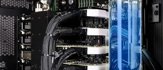
Designing a liquid cooling cold plate means solving conjugate heat transfer through the die, the thermal interface, the plate and the coolant, then trading peak junction temperature against pressure drop and pump power. CFD resolves the plate, a system model resolves the loop, and performance maps link the two.
Accelerator packages keep drawing more power and racks keep getting denser, so air runs out of headroom. Water carries roughly three thousand times more heat per unit volume than air, so direct-to-chip cooling takes the heat out at the source. It also raises questions that must be settled before cold plates, manifolds and coolant distribution units (CDUs) are frozen. Where are the hot spots, and does the channel layout follow them? What pressure drop can the pump afford? Does every plate in the rack get its flow? What happens when the workload steps?
How is a liquid cooling cold plate designed?
The heat path is a chain of resistances in series, and the coolant is the last link, not the end of the story.
- Junction to case. Heat leaves a die whose power map is strongly non-uniform. The hot spots, not the average flux, set the peak temperature, and the lid spreads them only partly.
- Thermal interface. A thin layer with a large temperature step: its bond-line thickness, flatness and ageing decide how much of the plate's capability ever reaches the die.
- Plate and fin conduction. Heat spreads through the base and climbs the fins. Wall thickness and fin efficiency decide how much of the wetted area does useful work.
- Channel convection. h = Nu k / D_h. In small laminar channels the flow is still developing, so Nu is high near the inlet and falls away; the layout decides where it is spent.
- Coolant temperature rise. The coolant warms by P / (ṁ c_p) on its way through, a floor no channel layout can remove; only more flow or a colder inlet lowers it.
- Manifolds and parallel plates. Plates in parallel share one pressure difference, so each gets the flow its own hydraulic resistance allows. A starved branch runs hot.
- CDU, pump and facility loop. The pump curve meets the loop's pressure-drop curve at the operating flow; the facility water sets the coolant inlet temperature.
Add the links and you have a budget: Tj ≈ Tin + P(Rjc + RTIM + Rplate + Rconv) + P/(ṁcp). The lumped chain shows which link dominates, but it cannot give the peak. A hot spot sees a local flux far above the package average, and heat spreads sideways through the lid and plate before it reaches the fluid. Conduction in the solids and convection in the coolant must be solved together. That is conjugate heat transfer, and on a real power map it is a 3D problem. Battery cold plates share much of the physics; see our article on EV thermal management simulation.
How do Reynolds, Prandtl and Nusselt numbers shape the channels?
The convection coefficient is h = Nu·k/Dh, with Nu set by Re = ρuDh/μ, by Pr = μcp/k and by the geometry. Cold-plate channels are small and the flow is mostly laminar. For fully developed laminar flow Nu is a constant of the cross-section and the thermal boundary condition (3.66 or 4.36 for a circular tube), so h rises only as Dh shrinks. Laminar Δp scales like μuL/Dh2, so thinner channels cost far more in pressure than they gain in h. That is the central trade of the design.
Developing flow complicates it. The thermal entry length is about 0.05·Re·Pr·Dh, and Pr is of order a few for water and higher for glycol mixtures. In short, dense fin arrays the flow is never fully developed, Nu is well above its long-duct value near the inlet, and correlations built for long ducts mislead. This is where resolved CFD earns its cost.
The hydraulics close the loop. Each plate has Δp = (fL/Dh + K)·ρu²/2, pump power is QΔp/η, and the pump's head–flow curve crosses the loop's pressure-drop curve at the operating flow. Change the plate and the crossing moves, and with it the flow every other plate receives.
Why does flow maldistribution make one plate run hot?
Plates in parallel share one supply-to-return pressure difference, but each tap sits at a different place along the manifold. Friction lowers the pressure along a header, momentum changes can raise it locally, and a plate with a higher resistance, a partial blockage or trapped air takes less flow. Unless the plate's own resistance dominates the manifold's, the branches are not fed equally, and the starved one runs hot. The OCP Cold Plate sub-project puts the technology cooling system "from the cold plate to the CDU" in scope, manifolds included, which is the right frame for the question.
Never optimise thermal resistance on its own
CFD or system simulation for liquid cooling: how are they linked?
Both, at different scales. The plate needs a resolved model; the loop needs a fast one.
| Scale | Model | The question it answers |
|---|---|---|
| Die, TIM, lid and cold plate | 3D conjugate CFD | Peak temperature on the real power map; R(Q) and Δp(Q) of the plate |
| Plates in parallel and manifolds | 3D CFD, or a 1D network with CFD-derived losses | Does every plate get the flow it was designed for? |
| Rack, CDU, facility loop, controls | 1D transient system model | Inlet temperature, flow and pump power over a workload, and failure cases |
| Air side of hybrid racks | CFD of the server and room | Does the air cooling of the remainder work? |
The two camps agree more than their headlines suggest. Modelon argues that CFD alone can no longer design a liquid-cooled system, yet calls it a key technology for cold-plate design and describes detailed component results being reduced to performance maps that feed the system model. Siemens notes that 1D system models run much faster than 3D CFD, so detailed CFD is reserved for where it matters most. Our view is the same: both, linked.
- Resolved CFD. A 3D conjugate model of one cold plate on its real power map: it resolves hot spots, developing flow and the channel layout.
- Planned runs. A designed set of CFD runs over flow rate, inlet temperature, power map and geometry variants, so the map covers the envelope without gaps.
- Performance map. Thermal resistance and pressure drop against flow, condensed from those runs into curves, tables or a surrogate with its validity limits stated.
- Rack and manifolds. A 1D network of plates in parallel, manifolds as loss elements and the pressure balance between branches, using the map as the plate component.
- Loop, CDU and controls. The pump, the heat exchanger, the facility water and the control logic, run transiently for load steps and pump or CDU failures at low cost.
- Bench calibration. Measured resistance and pressure-drop curves test the CFD and the map; the system model passes back flows and temperatures as new boundary conditions.
The map is not exotic. The OCP's Single-Phase Direct-to-Chip Cold Plate Test Specification 1.0.0 asks a bench for exactly its two curves. Thermal resistance is defined from the cold-plate base temperature, the inlet fluid temperature and the applied power, repeated at several flow rates. Pressure drop is measured at constant flow rates with the loop's tare subtracted and reported as a curve fit against flow. Make the CFD produce the same two curves, and the bench can test it while the system model consumes it. For workload transients, thermal-impedance curves from a CFD step response can be condensed into a small network of resistances and capacitances.
Why do cold-plate design iterations take so long?
A designer draws parallel or serpentine channels from experience. Each variant needs geometry clean-up, a fine channel mesh and a conjugate run, so only a handful are ever compared. A prototype then shows a hot spot that an average-flux assumption missed, or a pressure drop the pump cannot afford. By then the tooling is cut, the margin is spent on an oversized pump or a derated chip, and what was learned stays with whoever ran the test. Rack-scale experiments such as Heydari et al. (2024) in Applied Thermal Engineering show these quantities are measurable. They are simply measured late.
What can AI do for cold-plate design, and what can it not?
- Generative channel layouts that follow a non-uniform power map instead of a catalogue of straight or serpentine patterns.
- Surrogates of thermal resistance and pressure drop over geometry, flow, inlet temperature and power-map descriptors, trained on a planned set of CFD runs, with their own uncertainty. See surrogate models for CFD and FEA.
- Multi-objective optimisation of peak temperature, pressure drop, mass and manufacturability, with process limits as hard constraints. See generative design and optimisation.
- Calibration against the bench, tuning the uncertain inputs (interface resistance, roughness) and exposing where the model is wrong. See hybrid physics–AI modelling.
A 2026 preprint, Generative Design for Direct-to-Chip Liquid Cooling for Data Centers by Zheng Liu (University of Michigan-Dearborn), shows the first idea on the NVIDIA GB200 Grace Blackwell Superchip. A fast finite-difference thermal model scores each candidate, a constrained reaction–diffusion process generates channel topologies, and the loop repeats, shifting cooling toward the high-power regions. Against a baseline of parallel channels, the author reports reductions of more than 5 °C in average and more than 35 °C in maximum temperature.
Read it for what it is: a short conference paper whose evaluator is a 2D steady-state conduction model with a heat-transfer coefficient set by the channel mask. The results we found report temperatures, not pressure drop, flow distribution or measurements. The useful part is the method: generate, score quickly, iterate. To become a design tool, the scoring must include 3D conjugate CFD and the hydraulic cost.
Where AI does not help: a surrogate is only as good as the CFD that trained it, and it knows nothing outside its training envelope. It does not replace validation, and it should hand low-confidence questions back to the solver. See validation and benchmarking for how we keep those limits explicit.
Which coolant, and what about two-phase cooling?
The coolant sets Pr, viscosity and heat capacity, and so Re, Nu and Δp. The OCP publishes base specifications for cold-plate coolants for water-based, propylene glycol (PG 25) and two-phase dielectric fluids. Glycol raises viscosity, and so pressure drop, for the same channels. Two-phase adds latent heat, but also vapour quality and flow stability: multiphase territory that needs measurements before any model can be trusted.
From one cold-plate study to a design capability you keep
A single study answers the question it was asked. The larger return comes when the setup becomes a workflow your own team runs, so the next power map or manifold question costs hours, not weeks of manual set-up, and every answer is checked the same way. That is how we build liquid cooling work.
- Physics model. CFD and FEA set up once, as templates: geometry clean-up, mesh, solver settings and post-processing that every later run reuses.
- Validation. Mesh and time-step studies, and comparison with tests or full-scale data, so the model's uncertainty is known before it is trusted.
- Automated runs. Scripted runs over the parameters and operating conditions that matter, on your hardware or in the cloud.
- AI surrogate. A machine-learning model trained on those runs answers in seconds and says how sure it is; low-confidence questions go back to the solver.
- Decision tool. Optimisation, trade-off charts or operating guidance, in a form your engineers and operators use every day.
- Field data. Test, trial and monitoring data flow back to recalibrate the model, so it improves with every project instead of being rebuilt.
- An automated cold-plate template. Parametric geometry with the channel layout generated from a power map and your process limits as hard constraints, then meshing, conjugate set-up and post-processing of peak temperature, resistance and pressure drop.
- A validation record tying the model to your bench curves, with mesh studies and a stated uncertainty.
- Automated runs over flow, inlet temperature, power map and geometry.
- Performance maps and a surrogate, in the form your system model reads, with their limits written down.
- Training and handover, so your engineers can extend the workflow themselves. See our training and software development services.
Questions engineers ask about cold-plate liquid cooling
What is a cold plate in direct-to-chip liquid cooling?
Do I need CFD or a system simulation for liquid cooling?
How accurate is cold-plate CFD?
Can AI design the channel layout?
What do you need from us to start?
Our electronic systems cooling work and our AI/ML integration service cover this ground. If a cold plate, a manifold or a pump budget is on your desk, send us the power map, the stack-up and what you have measured. We will reply with how we would build the model, which bench data would validate it, and what the first results would let you decide. Start with a conversation.