Race car aerodynamics by CFD, from ride-height sweeps to wind-tunnel correlation
The tunnel slot is short, the model and the tunnel disagree on balance, and the lap-time team already runs on an aero map built from that CFD. A correlated, automated campaign on your own solver decides which points need the rolling road.
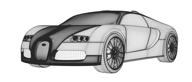
Race car aerodynamics by CFD predicts downforce, drag and aero balance at the ride height, pitch, yaw and flap settings the car really runs, and it is only as good as its moving ground, rotating wheels and separated wake. We build the workflow around your existing solver: a scripted aero-map campaign, a correlation record against your tunnel and track data, and a surrogate that states its range, so the next floor or wing update is a run your team launches, not a new project.
The tunnel slot is booked and the model is short. Which ride-height and flap combinations go on the rolling road, and which are left to CFD? If last season's model and tunnel agreed on drag and disagreed on front-to-rear balance, nobody can say whether mesh, turbulence model, ground simulation or tunnel was at fault. The lap-time team already runs on an aero map built from that CFD. A wrong guess costs a tunnel day, a late floor update or carbon parts cut to the wrong shape.
What makes race car aerodynamics hard to simulate?
Coefficients hide the difficulty. Force is F = ½ρU²A·C, so downforce and drag grow with the square of speed and a coefficient error is a force error in every corner. Balance, the share of downforce on the front axle, matters as much as the total: the authors of a 2026 race-car surrogate preprint call global balance at least as important as local peak loads.
Three mechanisms move the numbers. A floor and diffuser near the ground create suction that strengthens as the gap shrinks until the flow separates, so downforce is not a smooth function of ride height. A front wing in ground effect sheds a vortex system that manages the front wheel wake, and the floor pulls it inboard through an image vortex. Rotating wheels in ground contact shed wakes that feed the underfloor, so a small change at a wheelhouse moves loads on parts nobody touched.
Reynolds number adds a trap. The open Imperial Front Wing case, a three-element wing at 0.36 chords from the road, runs at a Reynolds number of 2.2 × 10⁵ on a 250 mm chord, so transition and separation belong to the answer, and an under-resolved solution lost features a finer one kept.
- Front wing in ground effect. A multi-element wing a fraction of its chord above the road loads the front axle and sheds a vortex system that the floor pulls inboard through its image and that manages the front wheel wake. A small change of ride height or flap angle moves those vortices, and with them the wake and the underfloor flow behind.
- Rolling road and rotating wheels. The road moves at the car's speed and the wheels turn with it. In CFD the ground and the tyre surfaces carry the same motion, the rim spokes are rotated and the tyre meets the road over a contact patch. A tunnel's belts and boundary-layer control differ from the open road, so the model must say which one it represents.
- Wheel wake. A rotating, loaded tyre sheds a wide, unsteady wake that feeds the underfloor and the flow to the rear wheels. Static wheels, a missing contact patch or a wrong ground condition change its width and the loads downstream, so the wheel treatment is validated, not assumed.
- Underfloor suction. Flow squeezed between floor and road speeds up and loses pressure, and that suction pulls the car towards the road: the downforce. It depends on the gap and on what enters it, so the front wing, the wheel wake and the attitude all act here.
- Ride height and attitude. Heave moves the whole floor towards or away from the road; pitch tilts it nose-down or nose-up. Each pairing is a different underfloor and a different wake, so each is one point of the aero map: a CFD run or a surrogate sample.
- Diffuser and separation. The rising floor lets the underfloor flow expand and recover pressure, which strengthens the suction ahead of it. If the expansion is too strong or the floor too low, the flow leaves the surface and a recirculation bubble forms. Separation is where steady RANS is least reliable and where a scale-resolving anchor earns its cost.
How do you model the rolling road and correlate with the wind tunnel?
A tunnel's rolling road is not the road. In the open Chalmers study of a full-scale DrivAer, the tunnel's five-belt system leaves no moving ground between front and rear wheels. Simulations that included the slotted-wall tunnel cut the average absolute drag error against the tunnel from 0.005 to 0.002 CD; open-road simulations overstated the drag change between open and closed rims by a factor of three for the slick and rain-grooved tyres. The authors point to tunnel blockage and to a ground system that changes how front wheel wakes reach the rear wheels.
So the ground condition is a modelling decision with a number attached. We set up both: an open-road domain with moving ground and rotating wheels for the map, and your tunnel's belts, struts and boundary-layer control for the correlation points, so a gap is assigned to the model or to the set-up. Wheels get a sliding mesh for the spokes, a rotating wall for the tyre and deformation under load; the radiator is a porous medium, so cooling drag sits inside the balance. A half-scale model at the same speed runs at half the Reynolds number.
Public data stops short. The AutoCFD DrivAer notchback case offers Pininfarina tunnel forces, pressures and velocity profiles, but with static wheels and a static floor. We check the workflow on the open DrivAer geometry from TU Munich, introduced in 2011 to bridge simple bodies and production cars, then repeat it on your tunnel data.
RANS or DES: what does each get wrong on separated flow?
Steady RANS with a k-ω SST model runs in hours and is the workhorse for a map. The authors of DrivAerML write that its correlation to measurements is unreliable for flows with large-scale separation, and name the rear notch and the underbody centreline as areas of strong scatter typical in CFD. They call delayed detached-eddy simulation, RANS in attached boundary layers and resolved eddies in separation, the most mature scale-resolving approach, with turnaround from overnight to a few days.
Resolution and statistics decide whether that cost buys anything. The DrivAerML runs use about 160 million cells and took around 40 hours on 1,536 cores, stopped automatically when the drag statistics reached ±1.5 drag counts (one count is 0.001 CD). The Chalmers runs averaged 17 flow passages to settle within 0.001 CD and put computational uncertainty at ±0.002 CD, against ±0.001 repeatability in the tunnel. We build those checks into the template, not into someone's memory.
We spend fidelity where it pays. Steady RANS covers the map; hybrid RANS-LES runs at anchor points and wherever separation is in doubt; the tunnel confirms the anchors. Increments are compared with increments: with the tunnel modelled, the Chalmers drag changes between tyre patterns fell within the uncertainty.
| Question | Model and setup | Known weakness | Decision it supports |
|---|---|---|---|
| Ride-height, yaw and flap sweep | Steady RANS, wall functions, moving ground, rotating wheels | Separation size and wake scatter | Which points get hybrid runs and tunnel time |
| Absolute downforce, drag and balance at anchors | Hybrid RANS-LES, statistical stopping | Over 100 million cells, long averaging | Level and balance of the aero map |
| Wheel, rim or tyre change | Hybrid, rotating wheels, tunnel domain | Domain choice changes the deltas | Wheel ranking from increments |
| Multi-element wing in ground effect | High-resolution scale-resolving, natural transition | Under-resolved runs lose vortices | Endplate, flap and canard changes |
| Radiator and cooling drag | Porous medium on the external flow | Pressure-drop data quality | Cooling against drag |
| Early concept screening | Surrogate trained on CFD, stated range | Smooths gradients, no extrapolation | Which concepts earn a full run |
How do you build an aero map without a thousand-run budget?
An aero map tabulates downforce, drag and balance over the attitude the car takes on track: front and rear ride height or heave and pitch, roll, yaw and steer, plus flap angles. A full grid of five parameters at five levels is 3,125 runs, so we use a space-filling design, add samples where the response bends, and tie the map to a few correlated anchor points.
Each run is a template: an attitude change that moves the body against the ground, an automated mesh, boundary conditions per case, statistical stopping, and a post-processor that writes forces, moments and balance to one table. The map feeds your vehicle dynamics simulation and lap-time tools directly.
- Attitude axes. The map is a table of downforce, drag and balance over the attitude the car takes. Front and rear ride height are drawn here; pitch, roll, yaw, steer and flap angle are further axes, taken as slices. Each cell is one run or one surrogate evaluation, and the contours are qualitative.
- CFD samples. A space-filling design, not a grid: the same number of runs covers every axis. The extra dots packed along the cliff are adaptive samples placed where the response bends fastest, and the few beyond it locate the edge instead of guessing it.
- Stall cliff. Downforce rises as ride height falls, then collapses where the underfloor or diffuser flow separates. The contours bunch towards it, and the section on the right shows the rise and the drop. The band is the scatter between models and tests, widest near the cliff.
- Correlation anchors. Hybrid scale-resolving runs and wind-tunnel points at chosen attitudes tie the level of the map to measurement. Their tolerances are set before the runs, and they sit where the map matters most, near the cliff and at the edges of the range.
- Surrogate range and gate. The dashed boundary encloses where the surrogate has training data and a stated uncertainty. A request outside it, or close to the cliff, goes back to the full solver instead of being answered by extrapolation.
- Track attitude path. A lap-time simulation reads the map along the attitude the car takes through braking, cornering and traction. The map is quasi-steady: it does not follow the motion itself. The ring marks where the path leaves the surrogate range and the gate hands that point to the solver.
A correlated map is evidence for a decision, not a guarantee of downforce or lap time
Where does AI help race car aerodynamics, and where does it not?
- A surrogate over the map. Trained on the designed runs, it returns forces and balance inside its range in seconds, and sends anything outside it or near the stall boundary back to the solver. In the preprint, a neural operator trained on a 625-sample race-car RANS dataset, each configuration run at six map points, predicted integrated drag and downforce to a mean error of 0.6% and 0.7% against the CFD. Thresholds were set in advance; drag met the usability threshold on all 20 parts and the stricter replacement threshold on 18.
- Concept screening. DrivAerNet++ holds 8,000 DrivAer variants in steady RANS. On a single-family test set the best of three deep-learning models reached a mean absolute CD error of 0.00691; across all body types, underbodies and wheels, R² fell to between 0.596 and 0.643 with errors of 0.0093 to 0.0104; the paper calls 0.005 against tunnel data acceptable.
- Correcting the physics. Both papers point to multi-fidelity tuning: sparse hybrid RANS-LES, tunnel and track points correcting a RANS-trained model.
It does not remove the physics. A surrogate inherits the RANS separation errors it was trained on and smooths sharp gradients, as the preprint reports at a splitter wing-tip. It does not extrapolate: the preprint marks a diffuser angle without training samples as out of domain. And a map is quasi-steady, silent on a car pitching through a braking zone. The physics model stays the evidence. See surrogate models for CFD and FEA, AI surrogate models you can sign off, and our surrogate modelling and uncertainty quantification pages.
From one aero study to a campaign your team can rerun
The return comes when the next floor, wing or ride-height question runs through the same chain.
- Physics model. CFD and FEA set up once, as templates: geometry clean-up, mesh, solver settings and post-processing that every later run reuses.
- Validation. Mesh and time-step studies, and comparison with tests or full-scale data, so the model's uncertainty is known before it is trusted.
- Automated runs. Scripted runs over the parameters and operating conditions that matter, on your hardware or in the cloud.
- AI surrogate. A machine-learning model trained on those runs answers in seconds and says how sure it is; low-confidence questions go back to the solver.
- Decision tool. Optimisation, trade-off charts or operating guidance, in a form your engineers and operators use every day.
- Field data. Test, trial and monitoring data flow back to recalibrate the model, so it improves with every project instead of being rebuilt.
- An attitude template in your solver: ride height, pitch, roll, yaw, steer and flap angle as inputs, ground and wheel treatment per case, a statistical stopping rule.
- A numerics standard with the grid, time-step and averaging studies behind each uncertainty figure.
- A correlation record against your tunnel and track data, tolerances set before the run, belt layout and blockage treatment written down.
- A campaign runner and post-processor that write the aero map in the format your lap-time tools read.
- A surrogate with a stated attitude range and a gate to the solver outside it.
- Handover and training, so your engineers run and extend it. See our training and software development services and the race car aerodynamics page.
Questions engineers ask about race car aerodynamics CFD
How accurate is CFD for race car downforce and drag?
Is RANS enough for an aero map, or do we need DES?
Does a correlated CFD model replace the wind tunnel or track test?
What is the DrivAer model and why validate on it?
How many CFD runs does an aero map need?
If an aero map or a tunnel plan is waiting on a decision, send us the attitude ranges you run, the tunnel set-up (model scale, belts, boundary-layer control), the correlation data you hold, and your solver. We reply with how we would design the campaign, the ground and wheel set-up, what the correlation record should contain, and what a surrogate could cover and where it would defer to the solver. Start with a conversation, or read the race car aerodynamics, automotive engineering and aerodynamics simulation pages.