ALE blast simulation: when it beats an empirical load, and when it does not
An empirical blast load assumes a clear path. When the structure shapes the wave, Euler-Lagrange coupling computes it. How the explosive, air mesh, coupling and structure fit together, how fine the cells must be, where coupling leaks, and when SPH, CFD or a curve is the better tool.
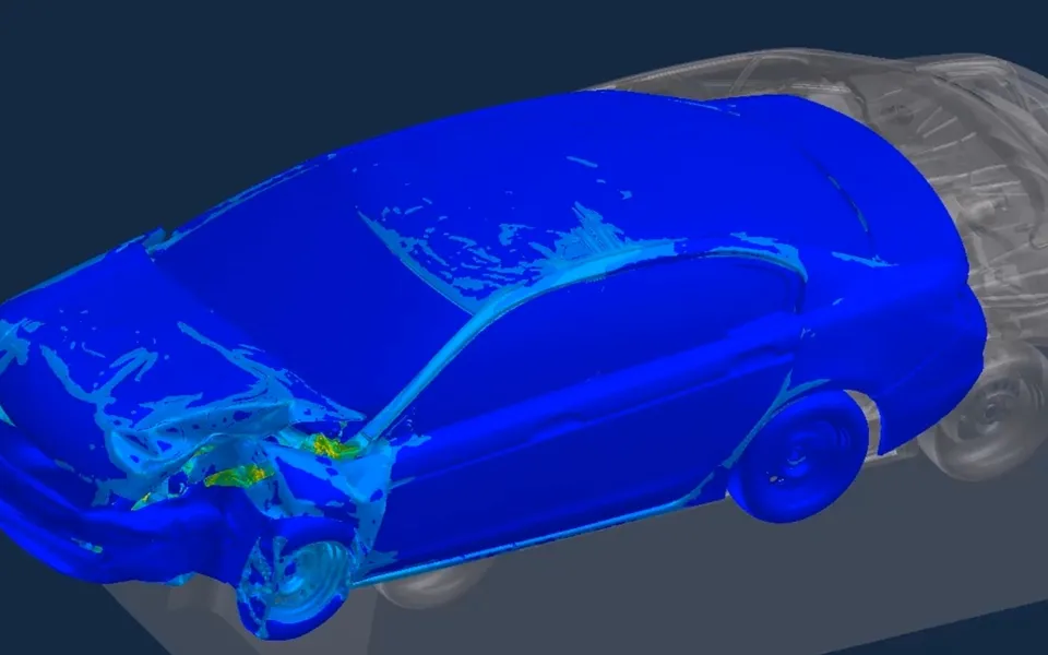
ALE blast simulation models the explosive and the air as Eulerian material flowing through a mesh, and couples that flow to a Lagrangian finite element structure, so the load is computed and not read from a curve. It earns its cost when the structure shapes its own load through reflection, diffraction, venting or close standoff, and it is the wrong first tool when a clear-path empirical load is enough. We build the model, its checks and the workflow on your explicit solver.
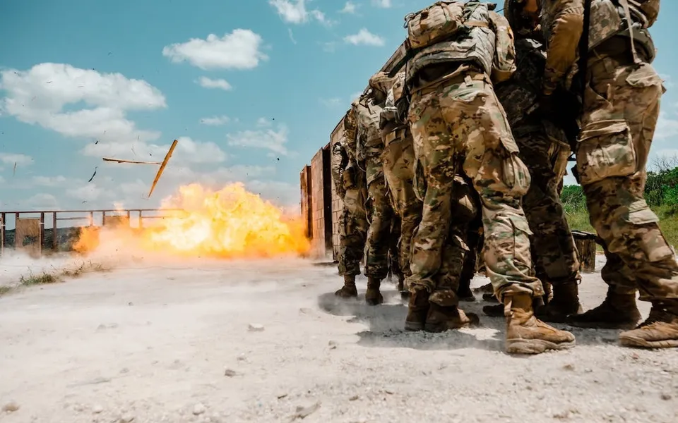
A blast-rated wall panel stands beside a re-entrant corner, and the load curve in the design guide knows nothing about the corner. The decision is the panel section and its connection: heavy and safe on paper, or lighter and defensible. Which load goes on the model, and how do you show it is right?
What does ALE blast simulation solve that an empirical load cannot?
An empirical load turns a charge mass and a standoff into a pressure-time history, scaled by Hopkinson-Cranz as Z = R / W1/3, with R the distance and W the equivalent TNT mass. Powell, Bogosian and Schwer (LS-DYNA Users Conference, 2018) say where it stops: the Kingery and Bulmash curves assume a spherical charge with a clear path and no reflections, lose accuracy at very close standoff, and LS-DYNA’s enhanced blast load keyword, which applies them, ignores shadowing and interior reflections from the target.
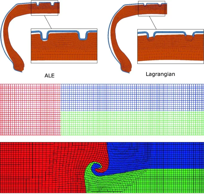
ALE computes the wave instead. The method goes back to Hirt, Amsden and Cook’s 1974 paper, where the mesh may move with the material, stay fixed or do anything between. In blast work the explosive and the air flow through their mesh, so violent motion near a detonation does not tangle cells, while the Lagrangian structure carries strain, plasticity and failure. LS-DYNA, Ansys Autodyn and Abaqus all offer this pairing.
Two equations of state carry the physics. Air is an ideal gas, p = (γ − 1)ρe. The explosive products follow the Jones-Wilkins-Lee form, p = A(1 − ω/(R1V)) exp(−R1V) + B(1 − ω/(R2V)) exp(−R2V) + ωE/V, with V the relative volume, E the internal energy per unit volume, and A, B, R1, R2 and ω constants fitted for each explosive. Lee, Hornig and Kury (UCRL-50422, 1968) chose them to match the measured detonation state and the expansion seen in the cylinder test.
How fine does the air mesh have to be to resolve a blast wave?
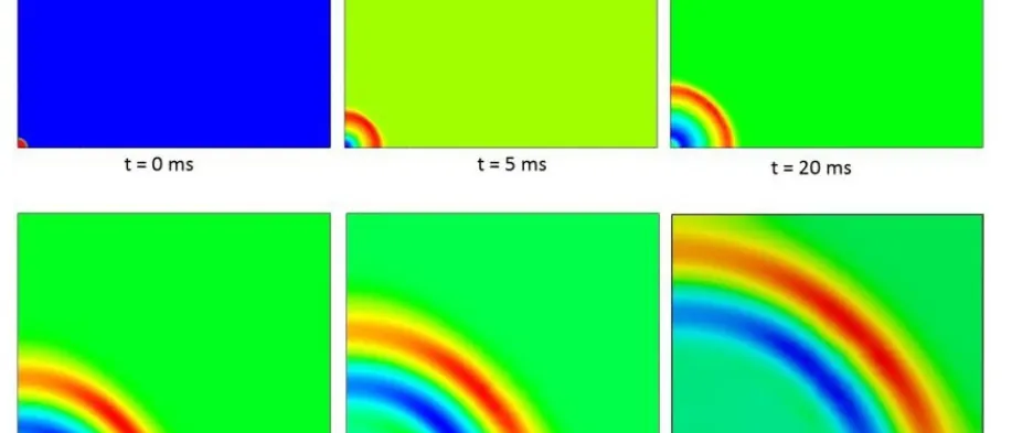
A shock cannot be thinner than a few cells, so cell size decides how much of the front survives. Powell et al. ran a spherical charge in air with LS-DYNA’s multi-material ALE solver and halved the cell size run by run. Larger cells gave a gradual rise and a lower peak, failed to separate the arrival of the shock from the detonation products, and lowered the impulse. Peak pressure was more sensitive than impulse, as Kuang and Liu (Heliyon, 2023) also note.
Both papers scale cell size as Hopkinson-Cranz scales distance: h = n W1/3, with n in mm/kg1/3. Powell et al. changed the charge mass by a factor of 8, scaled the gauge distance by 2, and found essentially identical convergence, so one study serves every charge at the same scaled standoff. Closer targets need finer meshes: for reflected impulse within 10 % of their finest result, their Table 1 gives maximum scaled cell sizes of 2.0, 4.8 and 6.4 mm/kg1/3 at scaled standoffs of 0.11, 0.33 and 0.66 m/kg1/3. That is one explosive, one rigid wall and one solver, so run your own study.
How do you map a 1D or 2D blast into a 3D model?
A fine 3D air mesh around a charge is expensive, so the early wave runs in a 1D or 2D axisymmetric model, where small cells are affordable. When the wave nears the structure, its pressure and velocity are mapped into the 3D air mesh and the structure is coupled. Powell et al. describe that sequence, and Kuang and Liu give different recommended coefficients for 1D, 2D and 3D models. The map needs its own check: Powell et al. cite a soil study in which a 3D mesh much coarser than the map lowered the peak, and say the effect in air needs further study. We compare the mapped load with the fine run before coupling.
- Front carried by fine cells. A pressure history at a gauge with a near-vertical rise and a high peak. A shock cannot be thinner than a few cells, so small cells keep it sharp.
- Front smeared by coarse cells. Larger cells give a gradual rise and a lower peak, and can merge the shock with the arrival of the detonation products that follow it. The wave arrives a little late.
- Cell size, scaled. At a gauge the rise time is about the time the front takes to cross a few cells. Scale the cell size with the cube root of the charge mass, as Hopkinson-Cranz scaling does for distance, and one convergence study serves every charge size at the same scaled standoff.
- Impulse. The area under the pressure history. It is less sensitive to cell size than the peak, and for close-in loads it is expected to control the response of most structural elements, but it still falls when cells are too coarse.
- Remap. The charge and the early wave run in a fine one- or two-dimensional axisymmetric model, which is cheap. Just before the wave reaches the structure, pressure and velocity are mapped into the three-dimensional air mesh.
- Three-dimensional air and structure. This mesh needs cells fine enough to carry the wave it receives, with the coupled structure inside it. Mapping into a much coarser mesh has been reported to lower the peak, so check the mapped load against the fine run.
Where does Euler-Lagrange coupling leak, and how do you know?
The air and the structure are different meshes, so they meet at coupling points, where air pressure becomes force on the structure and the structure’s velocity returns to the air, usually through a penalty stiffness. If the coupling is too soft or too sparse for the air cells, air passes through an intact wall and the structure sees too little load. Tan, Tay, Poon and Chng (2013) summarise the order of work for a column under close-in detonation: track the fluid to see whether leakage happens, set the coupling stiffness just high enough to stop it, and only if it persists switch on leakage control, keeping its forces small against the main coupling forces.
With solid-element structures there is no fluid inside, so leakage cannot be seen that way. The same authors suggest comparing coupling pressure on the surfaces with known solutions and proving the wave by mesh convergence: without correct incident pressure histories, reflected quantities are unlikely to be accurate.
- Explosive with a JWL equation of state. The charge is a material whose products obey a JWL pressure-volume-energy law. A burn model releases the energy as the detonation sweeps the charge, and the hot products then expand into the air.
- Eulerian air and the blast wave. The air is a mesh the gas flows through, so violent motion does not tangle cells. The shock is carried over a few cells, which is why the cell size sets the rise time and the peak.
- Coupling points. The fluid and the structure meet only here. Each point turns the air pressure into force on the structure and hands the structure's velocity back to the air, through a penalty stiffness that has to be tuned.
- Lagrangian panel. The structure keeps its own mesh, which moves and deforms with the material, so strain, plasticity and failure are tracked where they happen. As it bows it displaces the air and changes the load it receives.
- Leakage path. Where the coupling is too sparse or too soft for the air cells, air slips through an intact wall. The panel then sees too little load and pressure appears behind it for no physical reason.
- Gauges that expose it. Coupling pressure and force against a known solution, and pressure behind the wall while it is intact, show whether the coupling holds. Check them before reading a structural result.
Prove the free-field wave before you couple the structure
ALE, SPH, CFD or an empirical load: which is right for your case?
There is no single best method, as our page on numerical methods for blast, explosion and fire says. The choice follows from what the structure does to the wave and the wave to the structure; see also our ALE page and the blast, explosion and fire hub.
| Situation | Start with | Why | Check before you trust it |
|---|---|---|---|
| Clear path, no nearby surfaces, mid to far distance | Empirical load | The curves assume a clear path and are quick | Nothing reflects, shadows or confines the wave |
| Close-in standoff | ALE with an Eulerian charge | Powell et al. report the curves are less accurate below 0.4 m/kg1/3 | Cell size against scaled standoff |
| Reflection, diffraction, clearing, shadowing or interior reflections | Coupled ALE, or your existing CFD solver and a one-way load | The load depends on the geometry, which the curves ignore | The incident wave before coupling, and leakage |
| The structure deforms or fails enough to change the flow | Two-way coupled ALE | The load changes as the structure moves | Coupling stiffness, energy balance |
| Large open domain, many obstacles, and a structure that barely moves | Your existing CFD solver, pressure mapped on | Compressible CFD suits large domains | Resolution at each surface, impulse in the mapping |
| The structure’s own material breaks up and the pieces matter | SPH for the failing material | Particles carry the material, so no mesh tangles | Noise, boundaries, a Lagrangian run before failure |
Where does ALE blast simulation stop?
Simulation supports design decisions: choosing a section, connection or standoff, and planning the tests that confirm it. It does not certify, approve or rate a structure, or replace the test, safety study or competent-person sign-off that a regulator, an insurer or the owner’s process-safety function requires; acceptance of virtual evidence is agreed with that authority first. A converged model does not guarantee survival: it estimates the response to the load the hazard study chose.
How does machine learning help ALE blast work, and where does it not?
An ALE run is expensive, and the questions arrive in sweeps.
- Surrogate-assisted sensitivity. Scaled standoff, charge mass, panel thickness and scaled cell size go in; reflected impulse at the gauges, peak deflection and support reaction come out. A planned set of runs in LS-DYNA, Ansys Autodyn or Abaqus trains the surrogate, and its sensitivities rank what moves the response, with mesh error as a visible term. See surrogate models for CFD and FEA.
- Spending the expensive runs. Adaptive sampling adds runs where the surrogate is least certain or the response switches mode.
- Run triage. Energy balance, coupling pressure and the incident-wave check run after each job; a failing run never enters the training set.
It does not remove the physics. A surrogate inherits the error of every run it learns from, so an unconverged mesh gives a confident wrong answer, and it cannot cover a mode the runs never reached or tell you the coupling leaked. Outside its stated range, the full model answers. See AI surrogate models you can sign off and our page on fluid-structure interaction.
From one blast study to a blast-load capability you keep
The return comes when your engineers can put the next panel, standoff or enclosure through the same model, mesh study and checks without rebuilding them.
- Physics model. CFD and FEA set up once, as templates: geometry clean-up, mesh, solver settings and post-processing that every later run reuses.
- Validation. Mesh and time-step studies, and comparison with tests or full-scale data, so the model's uncertainty is known before it is trusted.
- Automated runs. Scripted runs over the parameters and operating conditions that matter, on your hardware or in the cloud.
- AI surrogate. A machine-learning model trained on those runs answers in seconds and says how sure it is; low-confidence questions go back to the solver.
- Decision tool. Optimisation, trade-off charts or operating guidance, in a form your engineers and operators use every day.
- Field data. Test, trial and monitoring data flow back to recalibrate the model, so it improves with every project instead of being rebuilt.
- A parametric ALE model in your existing explicit solver, with charge, standoff, mesh and coupling settings in a load-case file, not in the deck.
- A mesh-convergence script that scales cell size with the cube root of the charge mass and reports peak pressure and impulse at your gauge points.
- A free-field check and a coupling check on every job: incident wave against the reference, coupling force, pressure behind the intact wall, energy balance.
- A validation record against test or published data, with tolerances set before the run.
- An automated run set that plans the runs, submits them to your cluster and rejects any that fail the checks.
- A surrogate with a stated range and a gate that sends requests outside it to the full model.
- Handover and training, so your team extends it. See our training and software development services.
Questions engineers ask about ALE blast simulation
What is ALE in blast simulation?
Is ALE better than an empirical blast load?
What cell size does an air blast model need?
Should I use ALE or SPH for blast on a structure?
What do you need from us to start?
If an air blast load is holding up a panel, wall or enclosure specification, send us the geometry, the design basis that defines charge and standoff, your explicit solver and any test or published reference to match. We reply with how we would set up the ALE model and mesh study, which checks and tolerances the validation record should hold, and what a sweep over standoff and mesh would cover and where its range ends. Start with a conversation.