Power electronics thermal design: from mission profile to inverter lifetime
Traction inverters, chargers and drives are pushed to higher power density with SiC and IGBT modules. How electro-thermal models, 3D heat transfer and FEA, and AI surrogates predict the junction temperatures a mission will produce and the life they imply, before hardware.
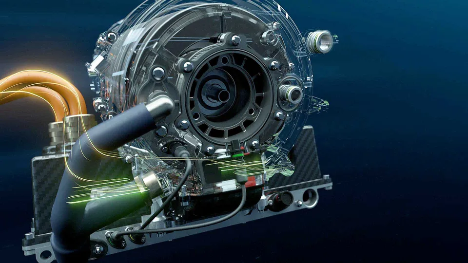
Power electronics thermal design means predicting the junction temperature, and above all its swings, that a real mission profile will produce, then turning those swings into a life with a model calibrated on power-cycling data. Compact thermal models give the temperature quickly, 3D heat transfer and FEA resolve the layout and the stresses where they cannot, and AI surrogates link the two.
Traction inverters, on-board chargers and grid and drive converters keep moving to higher power density, and wide-bandgap devices such as SiC allow higher switching frequency in smaller packages, so the same watts pass through less silicon area. The decisions that hang on the temperature are commercial: the current rating, how small the cooler can be, whether the warranty life holds over the real duty, and which substrate or attach technology to freeze before hardware exists.
What limits the lifetime of an inverter power module?
Mostly the packaging. Dragičević, Wheeler and Blaabjerg (2019) in IEEE Transactions on Power Electronics summarise it plainly: the most common failure modes are die-attach solder fatigue and bond-wire damage, and both are caused by junction-temperature cycles and the mean junction temperature of the device. For the broader physics-of-failure framing, see Wang et al. (2014) in IEEE Journal of Emerging and Selected Topics in Power Electronics.
The mechanism is a mismatch. The heat path from die to coolant is a stack of materials that expand by different amounts, and each warms by a different amount. A bonded joint of thickness h, with its far edge a distance L from the neutral point, sees a shear strain that scales like Δα·ΔT·L/h, where Δα is the mismatch in expansion coefficient. Repeat the cycle often enough and a crack grows from the corner of the die attach, a bond foot lifts, or the substrate delaminates at the edge of its copper.
- Junction and hot spots. Heat is generated in the active area of the die, and the junction temperature is the sum of the drops along the path below it. Chip-to-chip coupling and non-uniform current make some cells hotter than the average.
- Bond wires. Wires and ribbons carry current from the die to the substrate. They sit on a die that heats and cools, and the foot of the bond can lift off after enough temperature cycles.
- Die attach: solder or sinter. A thin layer joining two materials that expand differently, with a large temperature step across it. Shear strain concentrates at the edges and corners, where cracks start and grow inward.
- DBC substrate. Copper, ceramic, copper. The ceramic insulates and conducts heat, but it is stiff and expands little, so the copper edges are stressed and the bond between them can delaminate.
- Baseplate and its solder. The baseplate spreads heat sideways before the cooler, and it is joined to the substrate by another layer exposed to the same mismatch. It can warp as the module heats and cools.
- Thermal interface material. Fills the gap between module and cooler. Its thickness, flatness and ageing set a temperature step that can grow in service.
- Cooler and coolant. Convection and coolant temperature rise set the floor of the whole stack. Flow distribution decides whether every chip sees the same cooling.
How do you calculate junction temperature in an inverter?
Start with the coupling. Conduction loss depends on current and, typically, on temperature, because the on-state resistance of a MOSFET rises as the die warms; switching loss depends on voltage, current, frequency and temperature too. The temperature those losses produce feeds back into them, so the two are solved together, step by step.
The thermal side is usually a network, fitted to a measured or simulated step response as Zth(t) = ΣRi(1 − e−t/τi). A Foster network reproduces that curve with parallel RC stages, but its nodes are not physical layers, so you cannot change one layer and see the result. A Cauer ladder from the same response maps its stages onto the path from the die downward, which lets a designer ask what a thicker substrate does. Either way, the network is only as good as the cooling condition it was extracted at.
That is where compact models stop. They carry one heat path per chip, while real modules have lateral spreading in the copper and baseplate, neighbouring chips that heat each other, non-uniform current density, and a cooler whose flow is not the same under every chip. Those are three-dimensional conjugate heat transfer effects, the physics we describe for cold plates in AI accelerators and, on the vehicle side, for EV thermal management.
| Model | It answers | Where it breaks |
|---|---|---|
| Lumped Rth budget | Early sizing and comparison | No transients, spreading or coupling |
| Foster RC from a datasheet or test | Transients in a circuit simulation | Valid only at the fitted cooling condition; nodes are not layers |
| Cauer RC from 3D results or tests | Which layer carries the step; what a layer change does | One path per chip unless coupled |
| 3D conjugate heat transfer | Layout, spreading, chip coupling, hot spots, cooler flow | Too slow for a full mission, so it feeds the compact model |
| Thermomechanical FEA | Strain range per cycle at attach, bonds and substrate edges | Absolute life needs calibrated parameters |
How does cooler design change the temperature the die sees?
The cooler sets the floor of the whole stack. Convection in the channels or pin-fin field, the coolant temperature rise along the flow, and the interface between module and cooler add to every junction temperature, while spreading in the baseplate and the chip layout decide how evenly the chips share it. A cooler adequate on average can leave one chip position hotter. Where the coolant also serves the motor, the two interact: see our work on electric motor cooling and electronic systems cooling.
How do you turn a mission profile into inverter lifetime?
Run the loop. A mission profile, a drive cycle or a year of grid and ambient data, sets current, voltage and coolant temperature over time. The electro-thermal model turns it into a junction temperature history. Cycle counting, usually rainflow, reduces that history to swings, each with a range ΔTj, a mean Tjm and a duration. A lifetime model gives cycles to failure Nf for each swing, and Miner's rule adds the damage, LC = Σ ni/Nf,i. There are two kinds of cycle: slow swings from the mission, and fast swings within every current period.
- Mission profile. Speed and torque of a drive cycle, or grid and ambient conditions over months, turned into current, voltage and coolant temperature over time. The profile, not the rating, decides what the device lives through.
- Losses depend on temperature. Conduction and switching losses change with junction temperature, current, voltage and switching frequency, and the temperature they produce changes them again. The two must be solved together.
- Thermal response and the gate. A thermal-impedance network or a trained surrogate answers fast. If a question is outside its training range or its own uncertainty is wide, it is sent to 3D conjugate heat transfer and FEA instead.
- Temperature swings. The junction-temperature history is reduced by cycle counting to swings, each with a range, a mean and a duration.
- Damage. A lifetime model assigns each swing a number of cycles to failure, and a damage sum adds them up over the mission. The model's parameters come from power-cycling tests.
- Design change. Cooler, layout, interconnect, switching frequency or derating are changed, and the loop is run again until the life that the mission implies meets the target.
- Test data. Thermal-impedance measurements calibrate the thermal block and power-cycling results calibrate the lifetime model, with their scatter carried through to the answer.
The idea behind the lifetime model is old. Coffin–Manson says cycles to failure fall as a power law in the cyclic plastic strain range. Norris and Landzberg (1969) in the IBM Journal of Research and Development extended the idea for solder joints into a model that relates fatigue under one thermal cycling condition to another, so a test can stand in for the field. Power-module models keep that structure with temperature as the driver. The one Dragičević et al. use, taken from Scheuermann et al., has a power law in ΔTj, a term in the pulse duration and an Arrhenius term in Tjm, and its parameters come from experiments.
A life prediction is only as good as the temperature put into it
Qualification standards are where calibration data come from. The ECPE guideline AQG 324 defines a common procedure for module testing and for environmental and lifetime testing of power modules for automotive use. IEC 60749-34 (Semiconductor devices, power cycling) describes the power-cycling method: it cycles the power dissipated in the die and internal connectors, it is destructive, and it may not produce the same failure mechanisms as air-to-air temperature cycling. A pass is evidence about a test, not a prediction for your mission.
Where does thermomechanical FEA fit?
The thermal result is the load for the structural model. The 3D temperature field is mapped onto a finite element model of the stack, with elastic–plastic or creep behaviour for the attach layers, and the strain range per cycle at the critical corners feeds a fatigue relation. That is the thermomechanical chain we cover under thermal stress simulation and two-way thermal–structural coupling, with the time-dependent material behaviour in creep and creep–fatigue.
Comparing two layer stacks or attach technologies under the same cycle is robust, because the ranking survives many modelling uncertainties. An absolute life in years is not, until the damage parameters are calibrated on your own power-cycling data.
Where does AI help in power electronics thermal design, and where does it not?
- Surrogates of thermal impedance and peak junction temperature over layout and cooler parameters, trained on a planned set of 3D runs, with the surrogate's own uncertainty. See surrogate models for CFD and FEA.
- Fast mission-profile temperature prediction, so a year of operation becomes a quick evaluation feeding the lifetime estimate.
- Calibration with uncertainty from thermal tests and power-cycling data, so the life comes with a range. See uncertainty quantification and hybrid physics–AI modelling.
- Optimisation of cooler and layout against temperature swing, pressure drop and manufacturing limits.
Dragičević et al. show the architecture. One neural network maps operating conditions and design parameters, such as switching frequency and DC-link voltage, to thermal-stress variables, trained on experimental or simulation data. It converts the yearly mission profile into temperature swings, and a second network maps design parameters to yearly lifetime consumption. The authors report that evaluating the network was about four orders of magnitude faster than the look-up table it replaced, and used it to trade lifetime against filter size on a grid-connected PV converter.
The same paper is honest about its limits. The lifetime-model parameters were treated as fixed, and the authors leave their scatter, which would be handled by Monte-Carlo analysis, to future work. That is the data problem in one sentence. Temperature data cost compute; lifetime data cost test time and a destroyed device per point. So we let AI learn the temperature mapping and keep the lifetime relation a physical, calibrated model whose uncertainty is carried through. A surrogate also knows nothing beyond its training range, hence the gate that returns uncertain questions to the solver. See validation and uncertainty for AI surrogates.
From one module study to a thermal and lifetime workflow you keep
A single study answers the question it was asked. The larger return comes when the set-up becomes a workflow your own team runs, so the next substrate, cooler or mission profile costs hours, not weeks. That is how we build power electronics thermal and lifetime workflows.
- Physics model. CFD and FEA set up once, as templates: geometry clean-up, mesh, solver settings and post-processing that every later run reuses.
- Validation. Mesh and time-step studies, and comparison with tests or full-scale data, so the model's uncertainty is known before it is trusted.
- Automated runs. Scripted runs over the parameters and operating conditions that matter, on your hardware or in the cloud.
- AI surrogate. A machine-learning model trained on those runs answers in seconds and says how sure it is; low-confidence questions go back to the solver.
- Decision tool. Optimisation, trade-off charts or operating guidance, in a form your engineers and operators use every day.
- Field data. Test, trial and monitoring data flow back to recalibrate the model, so it improves with every project instead of being rebuilt.
- A parametric module template. Die, attach, substrate, baseplate, interface and cooler from a few parameters, meshed, solved for conjugate heat transfer and passed to a thermomechanical model.
- Compact thermal models condensed from the 3D results into RC networks your circuit simulator reads, with their valid conditions written beside them.
- A validation record tying the models to your measured cooling curves, with a stated uncertainty.
- A mission-profile pipeline from losses to temperature, cycle counting and damage, using your lifetime model and carrying its parameter scatter through.
- A surrogate with stated limits and a gate back to the solver.
- Training and handover: see our training and software development services.
Questions engineers ask about power electronics thermal design
Do I need 3D CFD, or is a thermal RC network enough?
Is a Coffin–Manson model enough to predict inverter lifetime?
How does SiC change the thermal design?
What do you need from us to start?
Our electronic systems cooling and thermal stress work and our AI/ML integration service cover this ground, within our thermal analysis and electromagnetic multiphysics capability. If a module, a cooler or a lifetime target is on your desk, send us the stack-up, the mission profile and what you have measured. We will reply with how we would build the model, which test data would validate it, and what the first results would decide. Start with a conversation.