Transfer path analysis that tells you which NVH path to fix first
A boom or a whine at the driver's ear is the sum of many paths. Blocked forces, FE and BE transfer functions, and hybrid and virtual TPA rank them, so the fix goes where it works, on the prototype or before one exists.
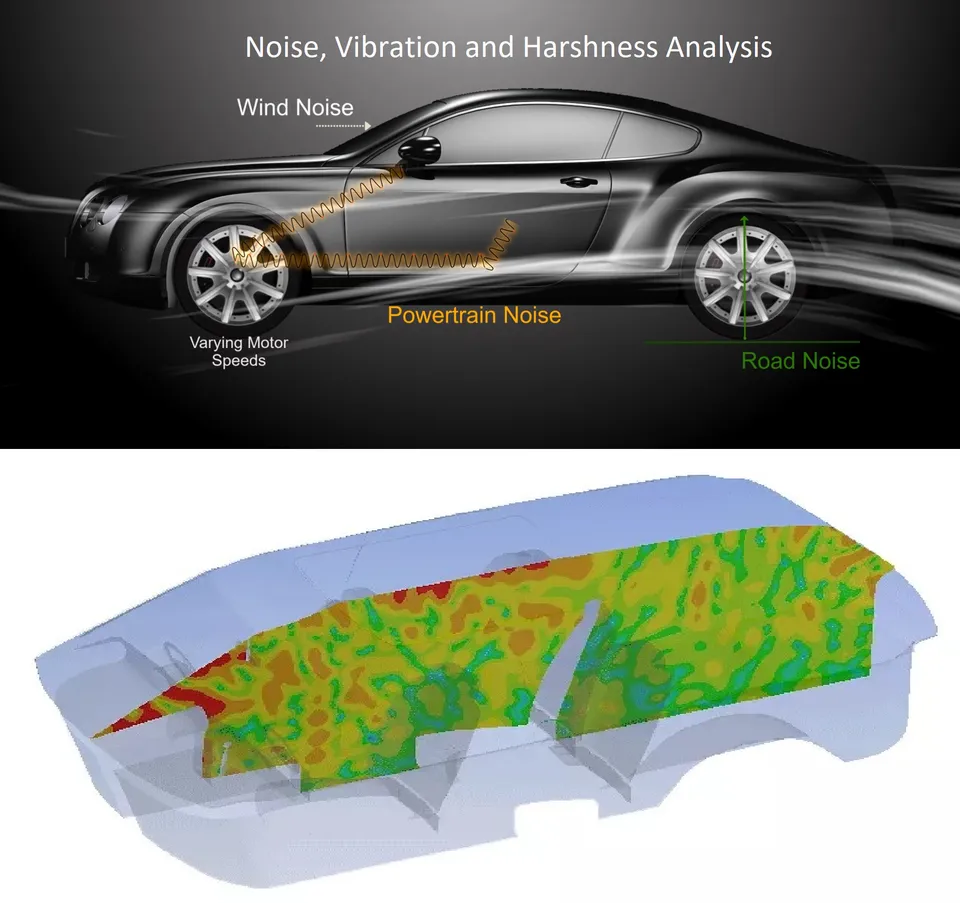
Transfer path analysis (TPA) splits the noise or vibration at a receiver, such as the driver's ear or a seat rail, into the contribution of every source and path, so you know which path to fix first. We build it from measured forces, FE and BE transfer functions, or a hybrid of both, as a workflow your team runs on every prototype and every design change, around your existing solvers.
The first integrated prototype has a boom in the cabin at one engine order on a steady cruise. The powertrain team measured the mounts and the unit meets its specification. The body team says the input is too high. The supplier says the same unit is quiet in other vehicles. Three fixes are on the table, a stiffer mount, a floor reinforcement and a damping treatment, and each costs a tool change or a build. Which path carries the boom decides which one pays.
What is transfer path analysis, and what does it tell you?
At one frequency the response at the receiver is a sum over paths. For structure-borne paths, p(ω) = Σ Hi(ω) Fi(ω): Fi is the force at interface point i, and Hi is the transfer function from that force to the response at the receiver. Airborne paths add terms of the same form, a source volume velocity qj times the acoustic transfer function from qj to the receiver. Every term is a complex number, so contributions add with phase. Two large paths can cancel, and removing one of them can make the cabin louder.
A TPA reports each term at the order or band that matters, and that is the ranking: “which path” becomes a number per path, not an argument between teams. Many variants exist. van der Seijs, de Klerk and Rixen, in Mechanical Systems and Signal Processing (2016) derive eleven from one framework and sort them into classical, component-based and transmissibility-based TPA. They differ in how the forces are obtained, and that choice decides what the ranking is worth.
- Source and its operating force. An engine, e-axle, compressor or pump shakes at orders of its speed. What leaves the source is a set of forces at its interface and, for airborne paths, a radiated sound field. Both are functions of operating condition.
- Structure-borne paths. Each mount, bush or link carries its own force F_i into the body. A, B and C are separate terms of the sum, and a path that carries more force is not always the path that matters at the receiver.
- Body transfer functions. H_i is the response at the receiver per unit force at interface point i. It holds the modes of the body and its damping, so it is large where a mode sits near the forcing order. This half of the problem is computed with an FE or BE model, or measured.
- Airborne path. Sound radiated by the source passes through firewall, floor, seals and trim. Its transfer function to the ear is obtained by reciprocity: a volume-velocity source at the ear, read at the panel.
- Receiver. The microphone at the ear or the sensor on a seat rail. The response is the complex sum of all path terms, p = sum of H_i F_i, so contributions add with phase and can cancel.
- Contribution ranking. Each path's term at the order of interest, side by side. The tallest bar is the first candidate for a fix, subject to what can be changed. Removing a path that was cancelling another makes the cabin louder.
Is the noise structure-borne or airborne?
Structure-borne paths carry force through mounts, bushes, links and fixings into the body, which then radiates sound as its panels move. Airborne paths carry sound from the source, through firewall, floor, seals and trim. Which one sets the level depends on the frequency, the source and the body, so it is computed per order and never assumed. In a test it is found by blocking or adding a path and listening. In a model it is a switch.
Panel-radiated and airborne transfer functions come cheaply by reciprocity: a volume-velocity source at the ear and the velocity read at the force point give the same transfer function as a force at that point and the pressure at the ear. One run with the source at the ear then covers every interface point and direction at once, in Nastran, Abaqus, Ansys or the acoustic solver Actran.
Why does classical TPA break on the forces?
The transfer functions are the easier half. The forces at an interface cannot be measured directly, because there is no place for a sensor between two bolted parts. There are three usual routes, each with a failure mode.
- Mount stiffness. Force is the dynamic stiffness of the mount times the displacement across it. It needs the dynamic stiffness at the operating preload, and it degrades where the displacement across the mount is small against the measurement error. Rotations are usually left out.
- Matrix inversion. Responses near the interface on the receiver side are multiplied by the inverse of a measured FRF matrix, F = H+ u. It needs more sensors than forces and a well-conditioned matrix. Near resonances, and with closely spaced paths, small errors become large forces of opposite sign on neighbouring paths.
- Blocked forces. The force that holds the source interface still, fbl, is a property of the source alone: it does not depend on the structure the source is mounted on. In situ it is found from fbl = Y+ u, with Y measured on the assembled structure. ISO 20270:2019 covers this indirect measurement. Its scope text sets the limits: vibration measured at all contact degrees of freedom, linear and time-invariant FRFs, and an on-board validation procedure for the quality of the result.
The real cost is time. Every route needs the vehicle, so the ranking arrives after the body is frozen and the repair is a late tool change. Scheuren and Lohrmann, in an SAE Brasil colloquium paper (2014) attribute TPA's slow acceptance as a standard tool partly to the measurement effort, and note that cutting measurements limits insight into the source mechanism and the accuracy of predictions. Fewer measurements need a validated model to supply what is missing.
How do hybrid and virtual TPA move the ranking before the prototype?
A blocked force belongs to the source, so it can be combined with any receiver. That one property gives two variants that fit a programme timeline. In hybrid TPA, forces come from a bench or the previous vehicle, and the transfer functions come from the FE and BE model of the new body. In virtual TPA, the forces come from a source model as well: a multibody or electromagnetic-structural model, as in our gear whine and flexible multibody work, or supplier data. This is substructuring, the framework reviewed by de Klerk, Rixen and Voormeeren (AIAA Journal, 2008): the source and the receiver are characterised apart and coupled at the interface.
The receiver model is where the work is. We build the trimmed body with damping that is measured, not guessed, the acoustic cavity, and the mounts as frequency-dependent elements. The interface is reduced to a few translations and rotations per mount, and it is calibrated against modal and FRF tests on the nearest existing body. The chassis side of the input follows from our vehicle dynamics and road-load work.
- Blocked force. The force a source exerts on its interface when the interface is held still, u = 0. It belongs to the source and does not change with the structure it is later mounted on. It is defined at the interface points, in translation and rotation.
- In-situ measurement. The source runs on a real assembly. Sensors near the interface record the operational response u, and the FRF matrix Y between interface and sensors turns it into forces, f_bl = Y+ u. More sensors than interface degrees of freedom make the inversion overdetermined and average out noise.
- Source property. The forces, per order or frequency line and operating condition, are stored with the sensor layout and inversion settings. One characterisation serves every later programme that uses the source.
- Any receiver. The same forces drive an FE, BE or measured model of body A or body B: p = sum of H f_bl. The body is replaced; the source record is not.
- Different bodies, different rankings. The contribution of each path depends on the receiver, so the path to fix first on body A may not be the one on body B. Computing both is a matter of a run, not a prototype.
- Held-out sensor. A sensor kept out of the inversion. The force set predicts its response, and the comparison with the measurement says whether the forces can be trusted. Large forces of opposite sign on neighbouring points point to an ill-conditioned inversion.
| What you have | Method | Forces come from | What to watch |
|---|---|---|---|
| A prototype, accessible mounts, a short deadline | Classical, mount stiffness | Mount dynamic stiffness and measured displacement | Preload dependence and left-out rotations |
| A prototype with stiff or buried joints | In-situ blocked force | FRF inversion on the assembled vehicle | Matrix conditioning, and a sensor held out of the inversion |
| A prototype, and no time for an FRF campaign | Operational, transmissibility-based | No forces, operational responses only | Less insight into the source mechanism |
| A new body in FE and a source already measured | Hybrid | Measured blocked forces on the FE and BE receiver | Receiver calibration and a matching interface |
| A source that does not exist yet | Virtual | Multibody or electromagnetic source models, or supplier data | Source model validation and its operating range |
| Many bodies, mount rates, orders and speeds | Surrogate-assisted | An automated run set feeding a trained surrogate | The stated design range, and a gate to the full model |
Validate the force set before you trust the ranking
Where does machine learning help TPA, and where does it not?
- Path ranking across variants. A surrogate of the contribution maps over mount rates, panel thickness and damping, trained on a planned set of FE and BE runs, ranks the paths for every candidate without a new run. See surrogate models for CFD and FEA.
- Sparse test data. A regularised, Bayesian inversion with the FE transfer functions as a prior returns blocked forces with their uncertainty from fewer sensors and impacts. A design-of-experiments step picks the sensor and shaker positions that carry the most information.
- FRF interpolation. Transfer functions measured on a coarse frequency grid or at a few points are filled in with a physics-constrained regression, so the model is calibrated on less data.
- Anomaly gates. Unit-to-unit outliers in the blocked-force library are flagged before they reach a ranking.
It does not replace the physics of the force. A network trained on operational data alone finds correlation, and paths driven by one shared source are correlated by construction, so it cannot tell which of them carries the energy. A surrogate has a stated range: outside the bush rates and body variants it was trained on, the request goes to the full model. The validation record is what lets you sign off the result. See AI surrogate models you can sign off.
From one path ranking to an NVH capability you keep
The return comes when your own team ranks the paths for the next body, mount layout or source without a new campaign.
- Physics model. CFD and FEA set up once, as templates: geometry clean-up, mesh, solver settings and post-processing that every later run reuses.
- Validation. Mesh and time-step studies, and comparison with tests or full-scale data, so the model's uncertainty is known before it is trusted.
- Automated runs. Scripted runs over the parameters and operating conditions that matter, on your hardware or in the cloud.
- AI surrogate. A machine-learning model trained on those runs answers in seconds and says how sure it is; low-confidence questions go back to the solver.
- Decision tool. Optimisation, trade-off charts or operating guidance, in a form your engineers and operators use every day.
- Field data. Test, trial and monitoring data flow back to recalibrate the model, so it improves with every project instead of being rebuilt.
- A parameterised receiver model in your existing solvers: trimmed body, acoustic cavity, mounts and named interface points, with reciprocal transfer-function runs scripted.
- A blocked-force library: one record per source and operating condition, with the sensor layout, the inversion settings and the validation result stored beside it.
- Automated contribution maps over speed, order and design change, ranking paths for every candidate body or mount rate.
- A correlation record tying modal, FRF and operational data to the model, with uncertainty stated.
- A surrogate with a stated range over the design variables you change, with a gate that returns out-of-range requests to the full model.
- Handover and training, so your engineers extend it themselves. See our training and software development services.
Questions engineers ask about transfer path analysis
What is transfer path analysis?
What is a blocked force?
What is the difference between classical, hybrid and virtual TPA?
Can TPA be done before a prototype exists?
What do you need from us to start?
If a boom, a drone or a harsh vibration is on your desk, send us the order and speed range, the mount layout, the body model or a description of it, and the operational spectra and FRFs you already hold. We will reply with how we would split the paths for your case, which TPA variant fits, what to measure and what to simulate, and what the first contribution ranking would let you decide. Start with a conversation, or read about our NVH simulation work and the acoustics and vibration section.